International Journal of Intelligence Science
Vol.05 No.05(2015), Article ID:60179,18 pages
10.4236/ijis.2015.55016
Compound Hidden Markov Model for Activity Labelling
Jose Israel Figueroa-Angulo1, Jesus Savage1, Ernesto Bribiesca2, Boris Escalante3, Luis Enrique Sucar4, Ron Leder3
1Biorobotics Laboratory, Universidad Nacional Autonoma de Mexico, Mexico City, Mexico
2Computer Science Department, Universidad Nacional Autonoma de Mexico, Mexico City, Mexico
3Electrical Engineer Department, Universidad Nacional Autonoma de Mexico, Mexico City, Mexico
4Computer Science Department, Instituto Nacional de Astrofisica, Optica y Electronica, Puebla, Mexico
Email: jifigueroa@uxmcc2.iimas.unam.mx, savage@servidor.unam.mx, bribiesca@iimas.unam.mx, borises@gmail.com, rleder@ieee.org, esucar@ccc.inaoep.mx
Copyright © 2015 by authors and Scientific Research Publishing Inc.
This work is licensed under the Creative Commons Attribution International License (CC BY).
http://creativecommons.org/licenses/by/4.0/


Received 3 August 2015; accepted 6 October 2015; published 9 October 2015
ABSTRACT
This research presents a novel way of labelling human activities from the skeleton output computed from RGB-D data from vision-based motion capture systems. The activities are labelled by means of a Compound Hidden Markov Model. The linkage of several Linear Hidden Markov Models to common states, makes a Compound Hidden Markov Model. Each separate Linear Hidden Markov Model has motion information of a human activity. The sequence of most likely states, from a sequence of observations, indicates which activities are performed by a person in an interval of time. The purpose of this research is to provide a service robot with the capability of human activity awareness, which can be used for action planning with implicit and indirect Human-Robot Interaction. The proposed Compound Hidden Markov Model, made of Linear Hidden Markov Models per activity, labels activities from unknown subjects with an average accuracy of 59.37%, which is higher than the average labelling accuracy for activities of unknown subjects of an Ergodic Hidden Markov Model (6.25%), and a Compound Hidden Markov Model with activities modelled by a single state (18.75%).
Keywords:
Hidden Markov Model, Compound Hidden Markov Model, Activity Recognition, Human Activity, Human Motion, Motion Capture, Skeleton, Computer Vision, Machine Learning, Motion Analysis

1. Introduction
In daily life, human beings perform activities to accomplish diverse tasks at different times throughout the day. These activities are made of one or several simpler actions which are performed at different times, and these simple activities have a chronological relationship to each other.
The motivation for this work is to analyse human behaviour by labelling the activities which are performed by a person. Human activity has the properties of being both complex and dynamic, since a person can be performing any action, which can be a pose or a motion, and change to another action.
The scope of this work is about presenting a method for labelling human activity. The pattern classification algorithm for the skeleton data uses an euclidean measure. The learning model uses a single large Hidden Markov Model, or Compound Hidden Markov Model, to tell the activities of a person from the output of the motion analysis.
The contribution of this work consists of two parts. Firstly, we present a novel way of computing features of a skeleton using distances between certain joints of both upper body and lower body. Secondly, we propose a Compound Hidden Markov Model for labelling cyclic and non-cyclic human activities; the Compound Hidden Markov Model is made of smaller Hidden Markov Models which connect to common states.
1.1. Activity Recognition
The taxonomy of human activities depend on the complexity of the activity [1] . A gesture is an elementary movement of a body part. Some examples of gestures are “waving an arm” or “flexing a leg”. Gestures are the building blocks for meaningful description of the motion of a person. An action is an activity performed by a single person, which is made of several gestures with chronological structure. The actions may involve interaction with objects. Some examples of actions are “walk” or “drink coffee”. An interaction is a human activity involving two or more persons and/or objects. For example, “two persons dance waltz” is an interaction between two persons, or “one person delivers a briefcase to other person” is an interaction between two persons and an object. A group activity is an activity performed by conceptual groups, composed of multiple persons and/or objects.
Some applications of the activity recognition are [1] : Domestic Robotics, where is used for interacting with a robot; in areas of Surveillance is used for detecting suspicious activity, analysing the activities performed in an room; the Gaming applications aim to achieve interaction with a video game without physical input devices; the Health Care area, where the activity recognition can be coupled to systems for emergency response or can be used for physical rehabilitation.
A particular use case for activity labelling on Domestic Robotics could be: for example, a robot helps in cooking. A person is preparing food in the kitchen. The vision system of the robot captures motion data of the person. The Activity Recognition System analyses the motion to get the activities performed. The output of the Activity Recognition System provides information to the Action Planning System, which has information of the world and the robot. The Action Planning System picks a plan of action, such as getting closer to the person and ask to help out.
There is a number of challenges on each stage of the activity recognition. When motion data is acquired, there is noise on the sensor, both from internal and external sources,which alters the captured values of the motion; the occlusion of the sensor by other objects or persons produces inaccurate or incomplete data. There are some issues which are exclusive of the Computer Vision-based systems: the orientation of the body towards the sensor can obscure some body parts, generating inaccurate or incomplete data; bad lighting conditions, if they are not compensated, reduce the accuracy of the capture. The challenges on classifying motion data are: the raw motion data can be high-dimensional, so picking the features which provide the best description is necessary; the position of the person in the motion data is not absolute, that is solved by making the motion data relative to a reference frame. The challenges when recognizing activities is that they can involve interaction with other persons or objects, this is solved by segmenting the data into separate entities and tracking them; several activities can have the same motion, which is solved by segmenting the motion data before training a classifica- tion model which provides the input for the recognition model.
1.2. Approaches to Activity Recognition
There are two approaches for activity recognition, according to how the motion data is represented and recognized [1] . The single-layered approach represents and recognizes human activities directly from sequences of images. This approach is suitable for gesture recognition and actions with sequential characteristics. In contrast, the hierarchical approach represents high-level human activities with a description in terms of simpler activities. This approach is suitable for analysing complex activities, such as interactions and group activities.
The taxonomy of the single-layered approach depends on the way of modelling human activities: space-time approach and sequential approach [1] .
The space-time approach views an input video as a three-dimensional (XYT) volume. This approach can be categorized further depending on the features used for the XYT volume: volumes of images [2] - [4] , volumes of trajectories [5] - [7] , or volumes of local interest point descriptors [8] - [10] .
The sequential approach uses sequences of features from a human motion source. An activity has occurred if a particular sequence of features which is observed after analysing the features. There are two main types of sequential approaches: exemplary-based and state model-based [1] . This work uses the state model-based approach to human activity recognition.
In the exemplary-based approach, human activities are defined as sequences of features which have been trained directly. A human activity is recognized by computing the similarity of a new sequence of features against a set of reference sequences of features, if a similarity is high enough, the system deduces that the new sequence belong to a certain activity. Humans do not perform the same activity at the same rate or style, so the similarity measuring algorithm must account for those details.
An approach to account for those changes is Dynamic Time Warping [1] [11] , a dynamic programming algorithm which stretches a pattern of motion over the time, to align and match it against a reference pattern of motion. The algorithm returns the cumulative distance between two patterns of motion. When comparing a pattern of motion against a set of reference patterns of motion, the reference pattern which has the highest similarity indicates the most likely activity [12] - [14] .
In the state model-based approach, human activities are defined as statistical models with a set of states which generate corresponding sequences of feature vectors. The models generate those sequences with a certain probability. This approach accounts for rate and style changes. One of the most used mathematical models for recognizing activities is the Hidden Markov Model [15] .
2. Hidden Markov Models
Hidden Markov Models, are statistical Markov Models in which the signal or process to model is assumed to be a Markov Process with unobserved states [15] . A stochastic process is a collection of random variables which represent the evolution of a random values over time, such as the spectra of a sound signal, or the probability of drawing a ball of a certain colour from a set of urns, which have coloured balls in varying amounts [15] .
The states in a stochastic process have the distribution probabilities for the collection of random variables, and the transitions from a state to other depend on probabilities (non-determinism).
The Markov property indicates that the probability distribution of future states depends upon the present state; in other words, it does not keep record of past time or future states (memoryless).
The unobserved states in a Hidden Markov Model indicate that the states are not visible directly, but output depends probabilistically on the state (Figure 1).
The most common applications of a Hidden Markov Model are temporal pattern recognition, such as speech recognition, handwriting recognition, gesture recognition, speech tagging, following of musical scores, and DNA sequencing.
The output values for the random variables in a Hidden Markov Model can be discrete, originated from a categorical distribution, or continuous, originated from a Gaussian Distribution.
The elements of a Hidden Markov Model (l) are: , where N, is the amount of states of the Markov process; M, is the amount of discrete output symbols for the Markov process; A, is the transition probability matrix between states of the Markov process; B, is the emission probability for output symbols per state of the Markov process; and
 , is the probability of starting at a certain state of the Markov process.
For a Hidden Markov Model to be useful in real world applications, three basic problems must be solved [15] :
Evaluation Problem: Given a sequence of observations  and a model
 , how to efficiently compute the probability of the sequence of observations, given the model
 ?
?
Optimal State Sequence Problem: Given a sequence of observations  and a model
 , how to choose the most likely sequence of states
  which describes best the sequence of observations?
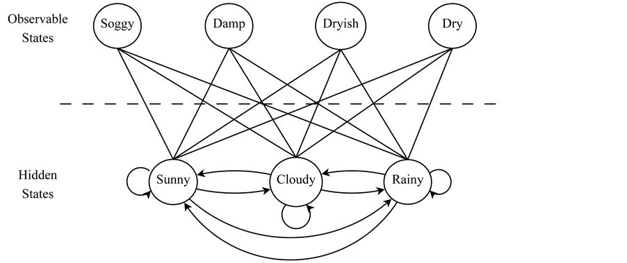
Figure 1. Hidden markov model.
Training Problem: How to adjust the parameters of the model  to maximize
 , the probability of a sequence of observations,
  , given the model?
2.1. Solution to the Evaluation Problem
The Forward Procedure solves the Evaluation Problem. The forward variable  defined as
 (1)
(1)
indicates the probability of the partial observation sequence,  , (until time t), and state
  at time t, given the model
 .
.
The inductive solution of  is the following:
1) Initialization:
 (2)
(2)
2) Induction:
 (3)
(3)
3) Termination:
 (4)
(4)
The initialization step sets the forward probabilities as the joint probability of state  and initial observation
 . The induction step computes the partial probability at the state
 , at time
  with the accompanying partial observations. And, the termination step computes the final forward probability by summing all the terminal forward variables
 .
.
2.2. Solution to the Most Likely Sequence of States Problem
The evaluation problem is solved by the Viterbi Algorithm, which computes the most likely sequence of connected states  which generates a sequence of observations
 , given a model
 .
.
The Viterbi Algorithm uses the variable , which contains the highest probability of a single path, at the time t.
 (5)
(5)
The highest probability along a single path, at time , is computed as:
 (6)
(6)
The most likely path is the sequence of these maximized variables, for each time t and each state j. The array  tracks all the maximized variables
 . The most likely state sequence is retrieved by backtracking the variable
 .
.
1) Initialization:
 (7a)
(7a)
 (7b)
(7b)
2) Recursion:
 (8a)
(8a)
 (8b)
(8b)
3) Termination:
 (9a)
(9a)
 (9b)
(9b)
4) Backtracking:
 (10)
(10)
2.3. Solution to the Training Problem
An approach for solving the Training Problem is the Viterbi Learning algorithm [16] , which uses the Viterbi Algorithm to estimate the parameters of a Hidden Markov Model. The algorithm can estimate the parameters from a set of multiple sequences of observations. That property makes it different of the Baum-Welch algorithm [15] , which requires all the training observation samples to be merged in a single sequence.
The initialization of the transition matrix is done with random values. The random values on each row are normalized, so its sum is equal to one. A bit mask matrix describing the transitions of a specific graph topology can be used to set the probabilities. The transition probabilities under a bit mask value equal to zero get a very small value, while the transition probabilities under a bit mask value equal to one get a random value.
The initialization step for the emission matrix uses one of these approaches: random values or segmented observation sequences. When initializing with random values, all the values must be larger than zero and each row must be normalized, so the sum of each row is equal to one. In the segmented observations sequences approach, the sequence is split by the number of states of the Hidden Markov Model. If the length of the sequence is not a multiple of the number of states, the last state gets less observations. For each state, the emission probability of each symbol is equal to the count of that symbol divided by the total amount of symbols assigned to that state.
The initial probability vector can be initialized either to uniform probabilities or by assigning the larger probability to an state or a number of states. The probabilities are normalized so its sum is equal to one.
In the induction step, for each sequence of observations for training, the Most Likely State Path is computed with the Viterbi Algorithm on the initial Hidden Markov Model, and the Likelihood Probability is computed either with the Viterbi Algorithm or the Forward Algorithm on the initial Hidden Markov Model. The Most Likely State Path of each sequence is stored for computing the parameters of an updated Hidden Markov Model. The Forward Probability of each sequence is accumulated in the variable  for computing the condition of termination.
The values of the updated transition matrix A are computed by counting the transitions from the state , to the next state
 , on the Most Likely State Paths associated to each sequence of observations for training. At the end, the values of each row on the transition matrix are normalized, so its sum is equal to one.
The values of the updated emission matrix B are the frequencies of each observation symbol in the observation sequence,  , per state in the Most Likely State Path,
  , at the time t, i.e.,
 . The values of each row on the emission matrix are normalized, so its sum is equal to one.
The initial probability vector  is updated by counting the states assigned to the first elements of each Most Likely State Path
 .
.
A new Hidden Markov Model is built from the updated model parameters . To check if the model maximizes
 , the Forward Probability of each sequence of observations for training is computed with the model, and accumulated in the variable
 .
.
The conditions for terminating the algorithm are: either the absolute of the difference of  and
and  is smaller than a threshold, or a certain number of iterations has been reached. If any of those conditions is false, the updated Hidden Markov Model is passed to the next iteration of the induction step, otherwise, the algorithm returns the updated Hidden Markov Model.
2.4. Logarithmic Scaling
Both Forward Probability Algorithm and Viterbi Algorithm store the result of floating-point operations in a single variable. The accumulated product of fractional values is a value so small that might fall below the minimum precision of the floating-point variable which stores the result. That variable can be represented in logarithmic scale, where multiplication and division operations are represented as addition and subtraction respectively. The range of values in logarithmic scale goes from , where negative logarithmic values represent fractional values and positive logarithmic values represent integral values larger or equal than one. In the case of the elements of a Hidden Markov Model, the values of A, B, and
  are converted to negative logarithmic values.
The logarithmic scale in the Forward Algorithm applies at each iteration in the Induction step, a scale variable accumulates the value of the forward variable , for each state. The forward probability is the sum of the logarithms of the scale for each state.
For the Viterbi Algorithm, the elements of the model  are converted to logarithmic scale. In the case of the emission matrix B, the emissions probabilities per states of each observation
  are converted to logarithmic scale. The value of the variable
  is updated by cumulative addition.
Hidden Markov Model Topologies
Depending on the process that generates a signal, the contents of the signal can have a stationary structure, or a chronological structure. The structure of the contents of the signal indicates which is the most suitable Hidden Markov Model [17] .
The classical case of the set of bowls containing different proportions of coloured balls is an example of a stationary process: any ball is drawn from any bowl at any time. For this case, the most suitable topology for the Hidden Markov Model is the ergodic model (Figure 2(a)), where all the states are fully connected [17] .
In automated motion recognition and activity recognition applications, the input data to be processed has a chronological or linear structure [17] .
The simplest topology for linear processes is the linear model (Figure 2(b)), where each states connects to itself (self-transitions) and to the next state. The self-transitions account for variations in the duration of the patterns in a state [17] .
The flexibility in the modelling of the duration can increase if it is possible to skip individual states in the sequence. One of the most used topology variations for automated speech and handwriting recognition is the Bakis model (Figure 2(c)). The Bakis model has a transition that skips two states ahead the current state, while the state is not the last state or the next-to-last state [17] .
The largest variations in the chronological structure are achieved by allowing a state to have transitions to any posterior states in the chronological sequence. The only forbidden transition is going from a state  to a state
  where
where . This model is called Left-to-Right model (Figure 2(d)) [17] .
Any of the Hidden Markov Models for signals with chronological structure―Linear, Bakis, Left-to-Right― can model cyclic signals by adding a transition from the last state to the first state (Figures 2(e)-(f)) [18] .
2.5. Related Work
The Hidden Markov Model is one of the most commonly used statistical models in the state model-based
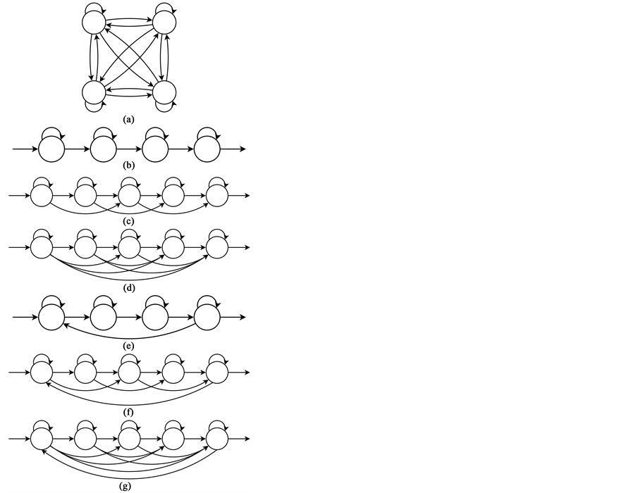
Figure 2. Hidden markov model topologies. (a) Ergodic HMM; (b) Linear HMM; (c) Bakis HMM; (d) Left-to-right HMM; (e) Cyclic linear HMM; (f) Cyclic bakis HMM; (g) Cyclic left-to-right HMM.
approach to Activity Recognition. There are two approaches for recognizing activities with Hidden Markov Models: Maximum Likelihood Probability (MLP) [19] - [23] and Most Likely State Path (MLSP) [24] - [28] . Next we list the main features, advantages and disadvantages of the two approaches.
2.5.1. Maximum Likelihood Probability Activity Recognition
• Features:
-Each Activity has a Hidden Markov Model.
-Each Hidden Markov Model computes the Forward Probability of a sequence of observation symbols.
-The Hidden Markov Model with the largest Forward Probability identifies the activity.
• Advantages:
-New activities can be added easily by training another Hidden Markov Model.
-The evaluation of a sequence of observation symbols can be performed by parallel tasks.
• Disadvantages:
-Motion segmentation is required when recognizing connected activities.
2.5.2. Most Likely State Path Activity Recognition
• Features:
-All the activities are embedded in a single large Hidden Markov Model.
-Each activity is represented by a subset of states.
-A sequence of observation symbols is processed to obtain the sequence of most likely states which generates it.
• Advantages:
-The evaluation of connected activities is possible without motion segmentation.
-Reconstruction of activities from the sequence of most likely states.
• Disadvantages:
-Adding a new activity is complicated: the Hidden Markov Model for the new activity is trained separately, the Hidden Markov Model is merged with the single large Hidden Markov Model and the single large Hidden Markov Model must be retrained to update the probabilities of emission and transition.
-The computation of likelihood probability with Viterbi Algorithm is slower than with Forward Algorithm,
-Reconstruction of activities requires an index which associates each activity with a subset of states.
2.6. Variants of Hidden Markov Models
A limitation of the Hidden Markov Models is that they do not allow for complex activities, interactions between persons and objects, and group interactions. To enhance the probability of recognizing activities with Hidden Markov Models, variations to the model have been studied in previous works.
In the Conditioned Hidden Markov Model [29] [30] , the selection of the states is influenced by an external cause. Such cause can be the symbols generated by an external classifier. The probability of those symbols in- creases the probability of a sequence. This model allows using two streams of different features from the same data.
The Coupled Hidden Markov Model [20] [31] [32] is formed by a collection of Hidden Markov Models. Each Hidden Markov Model handles a data stream. The observations cannot be merged using the Cartesian product of the amount of the symbols of each data stream. The nodes at the time t are conditioned by the nodes at the time  of all the related Hidden Markov Models. This model is suitable for recognizing activities using data from multiple sources.
The states of a Hidden Semi-Markov Model [33] - [35] emits a sequence of observations. The next state is predicted based on how long it has remained in the past state. This model relaxes the memoryless property of a Markov Chain.
The Maximum Entropy Markov Model represents [21] [36] the dependence between each state and the full observation system explicitly. The model completely ignores modelling the probability of the state . The learning objective function is consistent with the predictive function
 . The observation Y sees all the states X, instead of the observation being dependent on the state.
The Compound Hidden Markov Model [17] [37] - [40] is formed by the concatenation of sub-word units Hidden Markov Models. The sub-word units form a lexicon of words. Parallel connections link all the individual sub-word units. The recognized words are subsets of connected states in the most likely state path. The representation of the model can be simplified by the addition of non-emitting states.
The Dynamic Multiple Link Hidden Markov Model [41] is built by connecting multiple Hidden Markov Models. Each Hidden Markov Model models the activities of a single entity. The relevant states between multiple Hidden Markov Models are linked. This model is suitable for group activities.
The Two-Stage Linear Hidden Markov Model [42] is formed by two stages of Linear Hidden Markov Models. The first stage recognizes low-level motions or gestures to generate a sequence of gestures. The sequence of gestures becomes the input for the Hidden Markov Model at the second stage. The second stage recognizes complex activities from the sequences of gestures.
The Layered Hidden Markov Model [28] [43] is a model in which several Hidden Markov Models in layers of increasing activity levels. The layers at the lowest level recognizes simple activities. The simple activities form high-level activities at upper levels. The upper levels use the simple activities to recognize complex activities.
The Hidden Markov Model topology chosen for this work is the Compound Hidden Markov Model, because the purpose of this work is labelling activities performed by a person, during a period of time.
3. Proposed Approach
The method for activity recognition proposed in this work uses a representation of skeleton data based in Euclidean distance between body parts, and a Compound Hidden Markov Model for activity labelling.
3.1. Skeleton Features
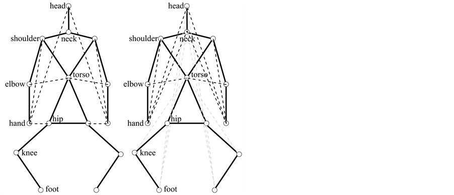
The features of the skeleton are a variation of those presented in Glodek et al. [30] . The features are made of set of Euclidean distances between joints. The work of Glodek et al., 2012 [30] represents poses from the upper body, as a set of Euclidean distances between these pairs of joints (Figure 3(a)): left hand-head, left hand-left shoulder, left hand-left hip, left elbow-torso, right hand-head, right hand-right shoulder, right hand-right hip, and right elbow-torso. This work uses a variation of the features described Glodek et al., 2012 to represent poses of the whole body, as a set of Euclidean distances between these pairs of joints (Figure 3(b)): left hand-head, left hand-neck, left hand-left shoulder, left elbow-torso, left foot-hip, left foot-neck, left foot-head, left knee-torso, right hand-head, right hand-neck, right hand-right shoulder, right elbow-torso, right foot-hip, right foot-neck, right foot-head, and right knee-torso.
3.2. Observations for the Hidden Markov Model
The observations for the Hidden Markov Model are computed from the Euclidean Distance between the features of two skeletons. To get the observations of a new sequence of motion data, the skeletons of each frame have their features computed. A set of similarities is computed for each frame of the new sequence of motion data. Those similarities come from the Euclidean Distance of the features of a frame of motion data and the features of each element of the codebook of key frames. The index of the key frame with the smallest Euclidean Distance becomes the observation of each frame.
3.3. Compound Hidden Markov Model
The model proposed for activity labelling is a Compound Hidden Markov Model [37] - [40] , which is a Hidden Markov Model where a subset of states represent a pattern, each subset of states is connected to a common initial state and a common final state, and the common final state always connects to the common initial state. The recognized patterns are extracted from the sequence of most likely states, obtained from applying the Viterbi Algorithm to a sequence of observations.
The Compound Hidden Markov Model is formed by several simpler Hidden Markov Models, whose topologies are configured according to the type of activity to model: the stationary activities, like sit still and stand still, have a single state; the non-periodic activities, like stand up and sit down, are modelled with Linear Hidden Markov Models; and, the periodic activities, such as walk, are modelled by a Cyclical Linear Hidden Markov Model.
 (a) (b)
Figure 3. Skeleton Features for pose description. (a) The work of Glodek et al., 2012 [30] represents poses from the upper body, as a set of Euclidean distances between the pairs of joints, which indicated by the black dashed lines; (b) This work uses a variation of the features described Glodek et al., 2012 to represent poses of the whole body, as a set of Euclidean distances between pairs of joints. The black dashed lines indicate the pairs of joints for the upper body, and the grey dashed lines indicate the pairs of joints for the lower body.
The activities are connected using context information. For example, the sit still activity connects to the first state of the stand up activity, and receives a connection from the last state of the sit down activity. The stand still activity connects to the first state of the sit down activity, and receives a connection from the last state of the stand up activity. Also, the stand still activity connects to the first state of the walk activity and receives a connection from the last state of the walk activity (Figure 4).
The stationary activities (sit still, stand still) are modelled with a Hidden Markov Model formed by a single state. The emission probabilities of each Hidden Markov Model are initialized to the averaged frequency of the observations for the corresponding idle activity.
The non-periodic activities (stand up, sit down) and the periodic activities, (walk), are trained using the following procedure: the observations from motion data of each activity are segmented into three sections: the anticipation (Figure 5(a)), which contains the poses which indicate that a motion is about to start; the action (Figure 5(b)), which contains the poses which describe a motion; and the reaction (Figure 5(c)), which contains the poses which indicate the recovery from an action to a neutral position. These three sections, anticipation- action-reaction (AAR), come from the theory of animation [44] [45] .
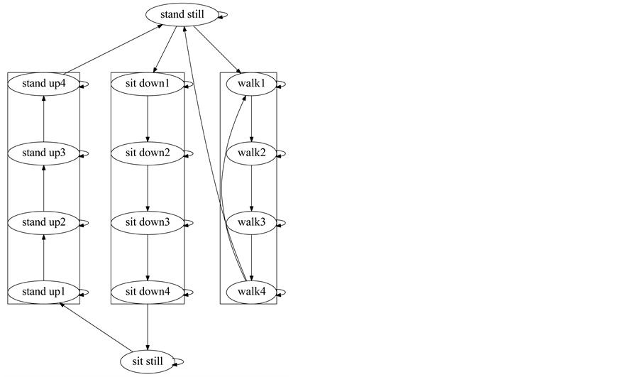
Figure 4. Compound hidden markov model for activity labelling.
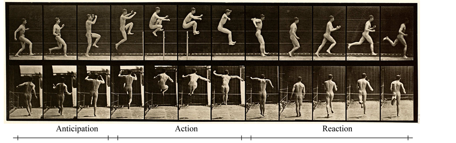
Figure 5. An activity has three sections: the motion preceding the activity (anticipation), the motion of the activity (action) and the motion after the activity is performed (reaction). Source: Animal Locomotion, Vol. 1, Plate 154, by Eadweard Muybridge, 1887.
The Hidden Markov Models for stationary activities, non-periodic activities, and periodic activities are merged in a Compound Hidden Markov Model, as specified in the Section 3.3, and its parameters are re- estimated using Viterbi Learning with all the elements of the training set.
4. Experiments
In order to assess the labelling accuracy of both the Compound Hidden Markov Model and some reference Hidden Markov Models, they was tested with a data set of human activities.
4.1. Data Source
The tests were performed using the Microsoft Research Daily Activity 3D Data set (MSRDaily) [46] , which was captured by using a Microsoft Kinect device.
The data set is composed by 16 activities, a) drink; b) eat; c) read book; d) call cellphone; e) write on a paper; f) use laptop; g) use vacuum cleaner; h) cheer up; i) remain still; j) toss paper; k) play game; l) lay down on sofa; m) walk; n) play guitar; o) stand up; and p) sit down which are performed by 10 persons, who execute each activity twice, once in standing position, and once in sitting position. There is a sofa in the scene. Three channels are recorded: depth maps (.bin), skeleton joint positions (.txt), and RGB video (.avi). There are  files for each channel. The whole set is formed by
  files. The position of the joints of the skeleton are computed from the depth map [47] .
For the purpose of this work, only the skeleton joint positions were used as input for labelling the actions, as well as a subset of activities: a) remain still (sitting pose) (Figure 6(a)); b) remain still (standing pose) (Figure 6(b)); c) walk (Figure 6(c) and Figure 6(d)); d) stand up (Figure 6(e) and Figure 6(f)); and e) sit down (Figure 6(g) and Figure 6(h)). Those activities are selected because there is a clear start in the sitting pose or the standing pose , or there are transitions between the sitting pose and the standing pose.
At the training step, the Hidden Markov Model is generated using a training set of motion data. The training set is made of the motion data from the first 6 subjects of the MSRDaily data set, while the motion data of the last 4 subjects constitute the testing set.
4.1.1. Computing the Codebook
The Microsoft Kinect sensor captures the depth map  of a motion sequence of an activity performed by a person. The depth map is processed to extract a skeleton
  [47] . During the
capture, a skeleton represents a single frame of the motion, therefore, a whole motion sequence contains several skeletons. The training set of an activity is formed by captures of motion sequences of the same activity performed by several people.
First of all, the skeletons have their features extracted, using the algorithm described in the Section 3.1. All the features from the skeletons of the training set are clustered with the k-means algorithm. The centroids of the clusters become the codebook of key frames.
The amount of symbols used in this work is 255, because that is the amount of symbols which provided the best labelling accuracy on the testing set, after performing tests on different amounts of symbols for the codebook, which were 31, 63, 127, 255, 511, 1023, 2047, and 4095 centroids1.
4.1.2. Building the Compound Hidden Markov Model
The Hidden Markov Model for a non-stationary activity has the following structure for its states: the amount of states is N, where , so the states can contain all the states of a motion; the state
  is for the random variables of the anticipation of the motion (Anticipation State), the state
  is for the random variables of the reaction of the motion (Reaction State), and the states
  are for the random variables of the action of the motion (Action States).
The transition probabilities from the Anticipation State to the Action States are initialized to uniform values. There are no transitions from the Action States to the Anticipation State. The transition probabilities from the
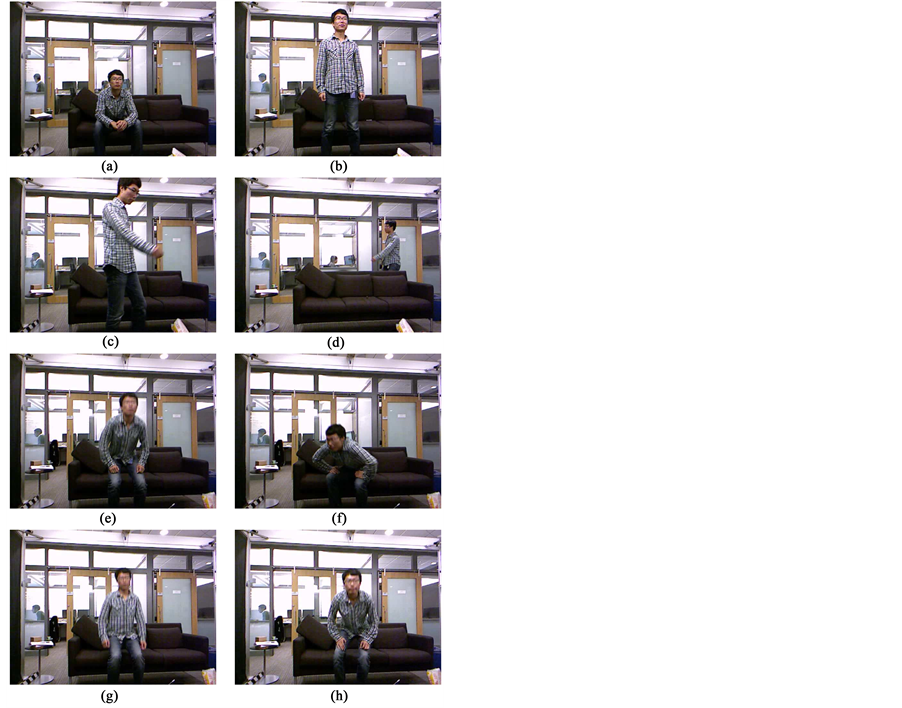
Figure 6. Subset of activities from Microsoft Research Daily Activity 3D used in this work. (a) Idle, sitting position; (b) Idle, standing position; (c) Walk in front of a sofa; (d) Walk behind a sofa; (e) Stand up, frontal orientation; (f) Stand up, three-quarters orientation; (g) Sit down, frontal orientation; (h) Sit Down, three-quarters orientation.
Action States to the Reaction State are initialized to uniform values. And, the transition probabilities from the Reaction State to the Anticipation State are set to uniform values.
The observations from the anticipation section are used for initialize the emission probabilities of the Anticipation State. The observations from the reaction section are used to initialize the emission probabilities of the Reaction State. The emission probabilities of the Action States are initialized to random values.
Both the transition probabilities and the emission probabilities for all the States will be refined after applying Viterbi Learning [16] to the Model.
4.2. Testing Activity Labelling.
The assessment of the quality of a labelled activity is done on the results of computing the Most Likely State Sequence from the observations of an activity.
The joints of the skeleton  are converted to vector of features
  (Section 3.1). The features
  are classified against a codebook of key frames
 , using Euclidean Distance.
The key frame with the minimum distance becomes an observation o, which is appended to a sequence of observations .
.
Assessing Labelling Accuracy
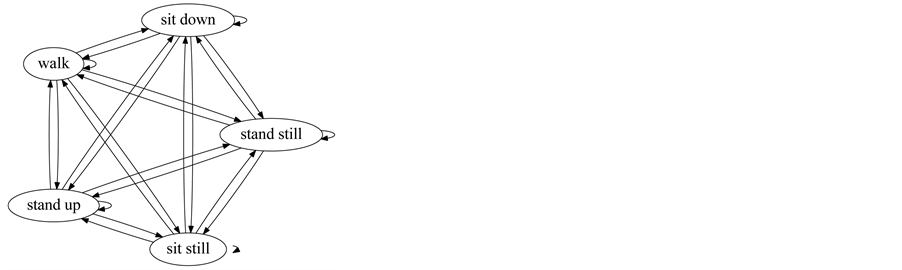
The first Hidden Markov Model to test is an Ergodic Hidden Markov Model where each state represent a single activity, giving a total of 5 states (Figure 7(a)).
 (a) (b)
Figure 7. Hidden markov models for activity labelling (reference). (a) Ergodic hidden markov model; (b) Graph-like hidden markov model.
For the second Hidden Markov Model, the proposal is a Hidden Markov Model organized like a Finite State Machine. Each activity is represented by a single state, giving a total of 5 states. The connections between the states of each activity use a language model.
The third Hidden Markov Model is a variation of the second Hidden Markov Model, where its parameters are retrained with Viterbi Learning. The connections between the states of each activity use a language model.
Both the second and the third Hidden Markov Model have a Graph-like structure (Figure 7(b)).
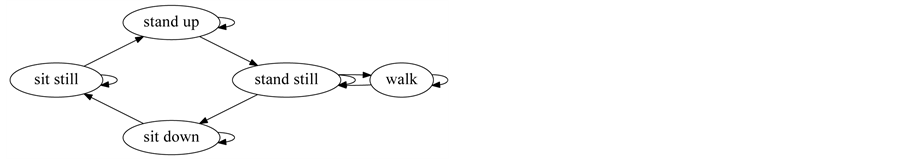
The fourth Hidden Markov Model is the Compound Hidden Markov Model proposed in the Section 2.3 (Figure 8). The connections between the states at the ends of each activity use a language model.
The language model for connecting coherent activities is the following:
•Sit Still ® Sit Still.
•Sit Still ® Stand Up ® Stand Still.
•Stand Still ® Stand Still.
•Stand Still ® Sit Down ® Sit Still.
•Stand Still ® Walk ® Stand Still.
The sequence of observations  is the input for the Compound Hidden Markov Model. The Viterbi algorithm decodes the sequence of observations to a sequence of most likely states
 . The states show an activity executed at an instant of time.
The criteria for determining the accuracy of the sequence of most likely states  is sequence accuracy. A sequence of states is accurate if the rate between the count of the states which follow the expected sequence of motions and the length of the sequence of states is greater or equal than a threshold of 90%. The language model for connecting coherent activities specifies the expected sequence of motions for an activity. Repeated states are allowed as long as they stay on a expected motion. The sequence accuracy criterion depends on the assessed activity (Table 1).
5. Results
The tests were performed on the four different Hidden Markov Models specified in the section 23. Each Hidden Markov Model was tested with the following amount of symbols 31, 63, 127, 255, 511, 1023, 2047, and 4095 , while keeping the amount of states of each Hidden Markov Model topology. The tables show the Hidden Markov Model with the amount of symbols that provided the highest labelling accuracy.
The assessed data was the sequence of most likely states  computed with the Viterbi Algorithm on the observations of the motion data. If all the states match the expected sequence of motions, the activity labelling is correct.
Table 2(a) and Table 2(b) show the average labelling accuracy of three codebook sizes for each topology of Hidden Markov Models which gave the highest labelling accuracy for all the activities. Tables 3(a)-(d) show the results of the tests on the 6 subjects of the training set from the MSRDaily data set. The first column shows the topology of the Hidden Markov Model, the columns 2-4 show the three sizes of codebooks which gave high accuracy for a first activity, and the columns 5-7 show three sizes of codebooks which gave high accuracy for a second activity.
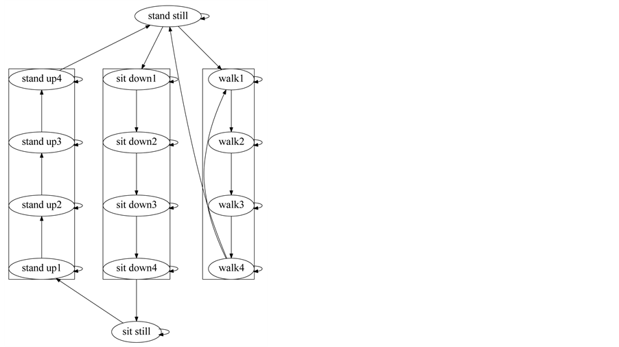
Figure 8. Hidden markov models for activity labelling (proposed). compound hidden markov model.

Table 1. Criteria for sequence accuracy per activity.
(a) (b)
Table 2. Average labelling accuracy for the hidden markov models with highest accuracy. (a) Training set, inter-joint distance features; (b) Testing set, inter-joint distance features.
(a) (b) (c) (d)
Table 3. Results on activity labelling accuracy for inter-joint distance features (training set). (a) Number of subjects, out of 6, with correct labelling on “sit” and “stand”; (b) Number of subjects, out of 6, with correct labelling on “walk” and “walk occluded”; (c) Number of subjects, out of 6, with correct labelling on “stand up 1” and “stand up 2”; (d) Number of subjects, out of 6, with correct labelling on “sit down 1” and “sit down 2”.
Tables 4(a)-(d) show the results of the tests on the 4 subjects of the testing set from the MSRDaily data set. The first column shows the topology of the Hidden Markov Model, the columns 2-4 show the three sizes of codebooks which gave high accuracy for a first activity, and the columns 5-7 show three sizes of codebooks which gave high accuracy for a second activity.
(a) (b) (c) (d)
Table 4. Results on activity labelling accuracy for inter-joint distance features (testing set). (a) Number of subjects, out of 4, with correct labelling on “sit” and “stand”; (b) Number of subjects, out of 4, with correct labelling on “walk”' and “walk occluded”; (c) Number of subjects, out of 4, with correct labelling on “stand up 1” and “stand up 2”; (d) Number of subjects, out of 4, with correct labelling on “sit down 1” and “sit down 2”.
The results for both the training set and the testing set show that the Compound Hidden Markov Model labels correctly a sequence of motion more often than an Ergodic Hidden Markov Model or the Graph-like Hidden Markov Models, when the amount of symbols is lesser than 2047 (Table 2(a) and Table 2(b)). The Compound Hidden Markov Model which had the highest labelling accuracy on the testing set has a codebook of 255 symbols.
In the Hidden Markov Models whose codebooks are of  symbols, the Retrained Graph-like Hidden Markov Model had a labelling accuracy similar to the Compound Hidden Markov Model (Table 2(a) and Table 2(b)).
It must be noted that the “Walk Occluded” activity is labelled incorrectly by all the Hidden Markov Models. The reason for such failure is that the skeleton data is incorrect or noisy because a sofa occludes the person who is walking. The algorithm which computes the skeleton [47] only works when the body is completely visible.
6. Conclusion
We present results for labelling human activity from skeleton data of a single Microsoft Kinect sensor. We present a novel way of computing features of a skeleton using distances between certain joints of both upper body and lower body. And, we propose a Compound Hidden Markov Model for labelling cyclic and non-cyclic human activities, which perform better than the reference Hidden Markov Models, an Ergodic Hidden Markov Model and a Graph-like Hidden Markov Model. The results for labelling 5 activities from 4 non-trained subjects show that the Compound Hidden Markov Model, with a codebook of 255 symbols, labels correctly a sequence of motion with an average accuracy of 59.37%, which is higher than the average labelling accuracy for activities of unknown subjects of an Ergodic Hidden Markov Model (6.25%), and a Compound Hidden Markov Model with activities modelled by a single state (18.75%), both with a codebook of 255 symbols. The contributions of this work are the representation of a full body pose with Euclidean distances between certain pairs of body joints, and the method for training a Compound Hidden Markov Model for activity labelling by segmenting the training data with the Anticipation-Action-Reaction sections from theory of animation. The future work involves using a new representation for the skeleton, based on Orthogonal Direction Change Chain Codes [48] [49] , for both the codebook and the input samples.
Acknowledgements
This work was supported by PAPIIT-DGAPA UNAM under Grant IN-107609.
Cite this paper
Jose IsraelFigueroa-Angulo,JesusSavage,ErnestoBribiesca,Luis EnriqueSucar,BorisEscalante, (2015) Compound Hidden Markov Model for Activity Labelling. International Journal of Intelligence Science,05,177-195. doi: 10.4236/ijis.2015.55016
References
- 1. Aggarwal, J. and Ryoo, M. (2011) Human Activity Analysis: A Review. ACM Computing Surveys, 43, 16:1-16:43.
http://dx.doi.org/10.1145/1922649.1922653 - 2. Bobick, A. and Davis, J. (2001) The Recognition of Human Movement Using Temporal Templates. IEEE Transactions on Pattern Analysis and Machine Intelligence, 23, 257-267.
http://dx.doi.org/10.1109/34.910878 - 3. Ke, Y., Sukthankar, R. and Hebert, M. (2007) Spatio-Temporal Shape and Flow Correlation for Action Recognition. Proceedings of the IEEE Conference on Computer Vision and Pattern Recognition, Minneapolis, 17-22 June 2007, 1-8.
http://dx.doi.org/10.1109/cvpr.2007.383512 - 4. Shechtman, E. and Irani, M. (2005) Space-Time Behavior Based Correlation. Proceedings of the IEEE Computer Society Conference on Computer Vision and Pattern Recognition, San Diego, 20-25 June 2005, 405-412.
http://dx.doi.org/10.1109/cvpr.2005.328 - 5. Campbell, L. and Bobick, A. (1995) Recognition of Human Body Motion Using Phase Space Constraints. 5th International Conference on Computer Vision, Cambridge, 20-23 June 1995, 624-630.
http://dx.doi.org/10.1109/ICCV.1995.466880 - 6. Rao, C. and Shah, M. (2001) View-Invariance in Action Recognition. In Proceedings of the 2001 IEEE Computer Society Conference on Computer Vision and Pattern Recognition, Kauai, 8-14 December 2001, II-316-II-322.
http://dx.doi.org/10.1109/cvpr.2001.990977 - 7. Sheikh, Y., Sheikh, M. and Shah, M. (2005) Exploring the Space of a Human Action. Proceedings of the Tenth IEEE International Conference on Computer Vision, Beijing, 15-21 October 2005, 144-149.
http://dx.doi.org/10.1109/iccv.2005.90 - 8. Ryoo, M.S. and Aggarwal, J. (2009) Spatio-Temporal Relationship Match: Video Structure Comparison for Recognition of Complex Human Activities. Proceedings of the 12th IEEE International Conference on Computer Vision, Kyoto, 27 September-4 October 2009, 1593-1600.
- 9. Wong, K.Y.K., Kim, T.-K. and Cipolla, R. (2007) Learning Motion Categories Using Both Semantic and Structural Information. Proceedings of the IEEE Conference on Computer Vision and Pattern Recognition, Minneapolis, 18-23 June 2007, 1-6.
http://dx.doi.org/10.1109/cvpr.2007.383332 - 10. Yilma, A. and Shah, M. (2005) Recognizing Human Actions in Videos Acquired by Uncalibrated Moving Cameras. Proceedings of the Tenth IEEE International Conference on Computer Vision, Beijing, 15-21 October 2005, 150-157.
http://dx.doi.org/10.1109/iccv.2005.201 - 11. Vintsyuk, T. (1968) Speech Discrimination by Dynamic Programming. Cybernetics, 4, 52-57.
http://dx.doi.org/10.1007/BF01074755 - 12. Darrell, T. and Pentland, A. (1993) Space-Time Gestures. IEEE Computer Society Conference on Computer Vision and Pattern Recognition, 335-340.
http://dx.doi.org/10.1109/cvpr.1993.341109 - 13. Gavrila, D. and Davis, L. (1996) 3-D Model-Based Tracking of Humans in Action: A Multi-View Approach. Proceedings of the IEEE Computer Society Conference on Computer Vision and Pattern Recognition, San Francisco, 18-20 June 1996, 73-80.
- 14. Yacoob, Y. and Black, M. (1998) Parameterized Modeling and Recognition of Activities. Proceedings of the Sixth International Conference on Computer Vision, Bombay, 7 January 1998, 120-127.
http://dx.doi.org/10.1109/iccv.1998.710709 - 15. Rabiner, L.R. (1989) A Tutorial on Hidden Markov Models and Selected Applications in Speech Recognition. Proceedings of the IEEE, 77, 257-286.
http://dx.doi.org/10.1109/5.18626 - 16. Rabiner, L. and Juang, B.H. (1993) Fundamentals of Speech Recognition. Prentice Hall, Englewood Cliffs.
- 17. Fink, G.A. (2007) Markov Models for Pattern Recognition: From Theory to Applications. Springer E-Books.
- 18. Magee, D.R. and Boyle, R.D. (2002) Detecting Lameness Using “Re-Sampling Condensation” and “Multi-Stream Cyclic Hidden Markov Models”. Image and Vision Computing, 20, 581-594.
http://dx.doi.org/10.1016/S0262-8856(02)00047-1 - 19. Chen, H.-S., Chen, H.-T., Chen, Y.-W. and Lee, S.-Y. (2006) Human Action Recognition Using Star Skeleton. Proceedings of the 4th ACM International Workshop on Video Surveillance and Sensor Networks, New York, 171-178.
http://dx.doi.org/10.1145/1178782.1178808 - 20. Starner, T.E. and Pentland, A. (1995) Visual Recognition of American Sign Language Using Hidden Markov Models. Proceedings of the International Workshop on Automatic Face-and Gesture-Recognition, Zurich, 26-28 June 1995.
- 21. Sung, J., Ponce, C., Selman, B. and Saxena, A. (2012) Unstructured Human Activity Detection from RGBD Images. Proceedings of the 2012 IEEE International Conference on Robotics and Automation (ICRA), Saint Paul, 14-18 May 2012, 842-849.
- 22. Xia, L., Chen, C.-C. and Aggarwal, J. (2012) View Invariant Human Action Recognition Using Histograms of 3D Joints. Proceedings of the 2nd International Workshop on Human Activity Understanding from 3D Data (HAU3D), Providence, 16-21 June 2012.
- 23. Yamato, J., Ohya, J. and Ishii, K. (1992) Recognizing Human Action in Time-Sequential Images Using Hidden Markov Model. Proceedings of the IEEE Computer Society Conference on Computer Vision and Pattern Recognition, Champaign, 15-18 June 1992, 379-385.
http://dx.doi.org/10.1109/cvpr.1992.223161 - 24. Bobick, A., Ivanov, Y., Bobick, A.F. and Ivanov, Y.A. (1998) Action Recognition Using Probabilistic Parsing. Proceedings of the IEEE Computer Society Conference on Computer Vision and Pattern Recognition, Santa Barbara, 23-25 June 1998, 196-202.
http://dx.doi.org/10.1109/cvpr.1998.698609 - 25. Nergui, M., Yoshida, Y., Imamoglu, N., Gonzalez, J. and Yu, W. (2012) Human Behavior Recognition by a Bio-\Monitoring Mobile Robot. In: Proceedings of the 5th International Conference on Intelligent Robotics and Applications—Volume Part II, Springer-Verlag, Berlin, Heidelberg, 21-30.
http://dx.doi.org/10.1007/978-3-642-33515-0_3 - 26. Oh, C.-M., Islam, M.Z., Park, J.-W. and Lee, C.-W. (2010) A Gesture Recognition Interface with Upper Body Model-Based Pose Tracking. Proceedings of the 2nd International Conference on Computer Engineering and Technology, Chengdu, 16-18 April 2010, V7-531-V7-534.
http://dx.doi.org/10.1109/iccet.2010.5485583 - 27. Yu, E. and Aggarwal, J.K. (2006) Detection of Fence Climbing from Monocular Video. In: Proceedings of the 18th International Conference on Pattern Recognition, IEEE Computer Society, Washington DC, 375-378.
http://dx.doi.org/10.1109/icpr.2006.440 - 28. Zhang, D., Gatica-Perez, D., Bengio, S. and McCowan, I. (2006) Modeling Individual and Group Actions in Meetings with Layered HMMS. IEEE Transactions on Multimedia, 8, 509-520.
- 29. Glodek, M., Layher, G., Schwenker, F. and Palm, G. (2012) Recognizing Human Activities Using a Layered Markov Architecture. In: Villa, A., Duch, W., érdi, P., Masulli, F. and Palm, G., Eds., Artificial Neural Networks and Machine Learning—ICANN 2012, Springer, Berlin, 677-684.
http://dx.doi.org/10.1007/978-3-642-33269-2_85 - 30. Glodek, M., Schwenker, F. and Palm, G. (2012) Detecting Actions by Integrating Sequential Symbolic and Sub-Symbolic Information in Human Activity Recognition. In: Proceedings of the 8th International Conference on Machine Learning and Data Mining in Pattern Recognition, Springer-Verlag, Berlin, Heidelberg, 394-404.
http://dx.doi.org/10.1007/978-3-642-31537-4_31 - 31. Brand, M., Oliver, N. and Pentland, A. (1997) Coupled Hidden Markov Models for Complex Action Recognition. IEEE Computer Society Conference on Computer Vision and Pattern Recognition, San Juan, 17-19 June 1997, 994-999.
http://dx.doi.org/10.1109/CVPR.1997.609450 - 32. Oliver, N., Rosario, B. and Pentland, A. (2000) A Bayesian Computer Vision System for Modeling Human Interactions. IEEE Transactions on Pattern Analysis and Machine Intelligence, 22, 831-843.
http://dx.doi.org/10.1109/34.868684 - 33. Duong, T.V., Bui, H.H., Phung, D.Q. and Venkatesh, S. (2005) Activity Recognition and Abnormality Detection with the Switching Hidden Semi-Markov Model. IEEE Computer Society Conference on Computer Vision and Pattern Recognition CVPR 2005, 1, 838-845.
http://dx.doi.org/10.1109/CVPR.2005.61 - 34. Natarajan, P. and Nevatia, R. (2007) Coupled Hidden Semi Markov Models for Activity Recognition. Proceedings of the IEEE Workshop on Motion and Video Computing, Austin, 23-24 February 2007, 10.
http://dx.doi.org/10.1109/wmvc.2007.12 - 35. Shi, Q., Wang, L., Cheng, L. and Smola, A. (2008) Discriminative Human Action Segmentation and Recognition Using Semi-Markov Model. Proceedings of the IEEE Conference on Computer Vision and Pattern Recognition, Anchorage, 24-26 June 2008, 1-8.
- 36. Sung, J., Ponce, C., Selman, B. and Saxena, A. (2011) Human Activity Detection from RGBD Images. Technical Report, Carnegie Mellon University, Department of Computer Science, Cornell University, Ithaca, NY.
- 37. Guenterberg, E., Ghasemzadeh, H., Loseu, V. and Jafari, R. (2009) Distributed Continuous Action Recognition Using a Hidden Markov Model in Body Sensor Networks. In: Proceedings of the 5th IEEE International Conference on Distributed Computing in Sensor Systems, Springer-Verlag, Berlin, Heidelberg, 145-158.
http://dx.doi.org/10.1007/978-3-642-02085-8_11 - 38. Lowerre, B.T. (1976) The Harpy Speech Recognition System. PhD Thesis, Carnegie Mellon University, Pittsburgh.
- 39. Ryoo, M.S. and Aggarwal, J.K. (2006) Recognition of Composite Human Activities through Context-Free Grammar Based Representation. Proceedings of the 2006 IEEE Computer Society Conference on Computer Vision and Pattern Recognition, New York, 17-22 June 2006, 1709-1718.
- 40. Savage, J. (1995) A Hybrid System with Symbolic AI and Statistical Methods for Speech Recognition. PhD Thesis, University of Washington, Seattle.
- 41. Gong, S. and Xiang, T. (2003) Recognition of Group Activities Using Dynamic Probabilistic Networks. Proceedings of the Ninth IEEE International Conference on Computer Vision, Nice, 13-16 October 2003, 742-749.
- 42. Nguyen-Duc-Thanh, N., Lee, S. and Kim, D. (2012) Two-Stage Hidden Markov Model in Gesture Recognition for Human Robot Interaction. International Journal of Advanced Robotic Systems, 9.
- 43. Oliver, N., Horvitz, E. and Garg, A. (2002) Layered Representations for Human Activity Recognition. In: Proceedings of the 4th IEEE International Conference on Multimodal Interfaces, IEEE Computer Society, Washington DC, 3-8.
http://dx.doi.org/10.1109/ICMI.2002.1166960 - 44. Lasseter, J. (1987) Principles of Traditional Animation Applied to 3D Computer Animation. ACM SIGGRAPH Computer Graphics, 21, 35-44.
http://dx.doi.org/10.1145/37402.37407 - 45. Williams, R. (2009) The Animator’s Survival Kit. Second Edition, Faber & Faber, London.
- 46. Wang, J., Liu, Z., Wu, Y. and Yuan, J. (2012) Mining Actionlet Ensemble for Action Recognition with Depth Cameras. Proceedings of the 2012 IEEE Conference on Computer Vision and Pattern Recognition (CVPR), Providence, 16-21 June 2012, 1290-1297.
http://dx.doi.org/10.1109/cvpr.2012.6247813 - 47. Shotton, J., Fitzgibbon, A., Cook, M., Sharp, T., Finocchio, M., Moore, R., Kipman, A. and Blake, A. (2011) Real-Time Human Pose Recognition in Parts from Single Depth Images. In: Proceedings of the 2011 IEEE Conference on Computer Vision and Pattern Recognition, IEEE Computer Society, Washington DC, 1297-1304.
http://dx.doi.org/10.1109/cvpr.2011.5995316 - 48. Bribiesca, E. (2000) A Chain Code for Representing 3D Curves. Pattern Recognition, 33, 755-765.
http://dx.doi.org/10.1016/S0031-3203(99)00093-X - 49. Bribiesca, E. (2008) A Method for Representing 3D Tree Objects Using Chain Coding. Journal of Visual Communication and Image Representation, 19, 184-198.
http://dx.doi.org/10.1016/j.jvcir.2008.01.001
NOTES

1The reason for those sizes for the codebooks was that for the experiments, the initial amount of symbols were powers of two―32, 64, 128, 256, 512, 1024, 2048, and 4096―but one of the centroids computed by the k-means algorithm had undefined values (NaN values) and had to be removed from the codebook, to avoid arithmetical errors when computing the Euclidean distance between any data object and a centroid with undefined values.