International Journal of Intelligence Science
Vol.2 No.1(2012), Article ID:17034,8 pages DOI:10.4236/ijis.2012.21001
Evaluating Effects of Two Alternative Filters for the Incremental Pruning Algorithm on Quality of POMDP Exact Solutions
Computer Science Department, Texas Tech University, Lubbock, USA
Email: mahdi.moghadasi@ttu.edu
Received September 11, 2011; revised October 1, 2011; accepted October 12, 2011
Keywords: Planning Under Uncertainty; POMDP; Incremental Pruning Filters
ABSTRACT
Decision making is one of the central problems in artificial intelligence and specifically in robotics. In most cases this problem comes with uncertainty both in data received by the decision maker/agent and in the actions performed in the environment. One effective method to solve this problem is to model the environment and the agent as a Partially Observable Markov Decision Process (POMDP). A POMDP has a wide range of applications such as: Machine Vision, Marketing, Network troubleshooting, Medical diagnosis etc. In recent years, there has been a significant interest in developing techniques for finding policies for (POMDPs).We consider two new techniques, called Recursive Point Filter (RPF) and Scan Line Filter (SCF) based on Incremental Pruning (IP) POMDP solver to introduce an alternative method to Linear Programming (LP) filter for IP. Both, RPF and SCF have solutions for several POMDP problems that LP could not converge to in 24 hours. Experiments are run on problems from POMDP literature, and an Average Discounted Reward (ADR) is computed by testing the policy in a simulated environment.
1. Introduction
One of the most challenging tasks of an intelligent decision maker or agent is planning, or choosing how to act in such of interactions with environment. Such agent/environment interactions can be often be effectively modelled as a Partially Observable Markov Decision Process (POMDPs).Operation research [1,2] and stochastic control [3] are two domains where this model can be applied for balancing between competing objectives, action costs, uncertainty of action effects and observations that provide incomplete knowledge about the world. Planning, in the context for a POMDP, corresponds to finding an optimal policy for the agent to follow. The process of finding a policy is often referred to as solving the POMDP. In the general case, finding an exact solution for this type of problem is known to computationally intractable [4,5]. However, there have been some recent advances in both approximate and exact solution methods.
In some cases, an agent does not need to know the exact solution of a POMDP problem to perform its tasks. Over the years, many techniques have been developed to compute approximate solutions to POMDP problems. The goal of finding approximate solutions is to find a solution in a fast way within the condition that it does not become too far from the exact solution.
Point-based algorithms [6-8] choose a subset of B of the belief points that is reachable from the initial belief state through different methods and compute a value function only over the belief points in B. After the value function has converged, the beliefpoint set is expanded with all the most distant immediate successors of the previous set.
PBVI and Perseus use two opposing methods for gathering the belief point sets B. In larger or more complex domains, however, it is unlikely that a random walk would visit every location where a reward can be obtained. PBVI attempts to cover the reachable belief space in a uniform density by always selecting immediate successsors that are as far as possible from the B. Perseus, on other hand, simply explores the belief space by performing random trajectories. While the points gathered by PBVI generate a good B set, the time it takes to compute these points makes other algorithms more attractive.
However, approximate methods have the drawback that we cannot precisely evaluate them without knowing the exact solutions for the problems that we are solving. Furthermore, there are crucial domains that need exact solution to control accurately. For example when dealing with human’s life or controlling an expensive land rover. Our objective in this paper is to present an alternative solver to evaluate approximate solutions on POMDP problems with small number of states.
Among current methods for finding exact solutions, Incremental Pruning (IP) [9] is the most computationally efficient. As with most exact and many approximate methods, a set of linear action-value functions are stored as vectors representing the policy. In each iteration of running algorithm, the current policy is transformed into a new set of vectors and then they are filtered. The cycle is repeated for some fixed number of iterations, or until the value function converges to a stable set of vectors, The IP filter algorithm relies on solving multiple linear programs (LP) at each iteration. We consider two new techniques, called Recursive Point Filter (RPF) and Scan Line Filter (SCF) based on Incremental Pruning (IP) POMDP solver to introduce an alternative method to Linear Programming (LP) filter. More details about this method will be explained later.
2. POMDP Problem
2.1. Background
Planning problem is defined as: given a complete and correct model of the world dynamics and a reward structure, find an optimal way to behave. In Artificial intelligence, when the environment is deterministic our knowledge about our surrender describes with set of preconditions. In that case, Planning can be addressed by adding those additional knowledge preconditions to traditional planning systems [10]. However in stochastic domains, we depart from the classical planning model. Rather than taking plans to be sequences of actions, which may only rarely execute as expected, we take them to be mapping from states—which are situations—to actions that specify the agent’s behaviour no matter what may happen [11].
2.2. Value Function
The value iteration algorithm for POMDP was introduced by [2] first. The value function V for the belief-space MDP can be represented as a finite collection of |S|—dimensional vectors known as α vectors. Thus, V is both piecewise—linear and convex [2]. Although its initial success for solving hard POMDP problems, there are two distinct reasons for the limited scalability of a POMDP value iteration algorithm. The more widely reason is dimensionality [12]; in a problem with n physical states, POMDP planners must reason about belief states in an (n – 1) dimensional continuous space. The other reason is, the number of distinct action—observation histories grows exponentially with the planning horizon. Pruning is one proposed [9] solution to whittle down the set of histories considered.
Value functions are represented by vectors in R|S|, where each element s ∈ S of a vector represents the expected long term reward of performing a specific action in a corresponding state s. As the agent does not fully know the state it is currently in, so it would value the effect of taking an action depending on the belief it has for the existing states. This results in a linear function over the belief space for each vector. In other words, the value function simply determines the value of taking an action a given a belief b that determines the probability distribution over S. For example, in a simple problem with two states, if taking action a costs 100 in state s1, and –50 for s2 , then if the agent believes 50% to be in s1, then the value of performing a would be valued as 25. Thus, it can be formulated as mapping from the belief space to a real number, which is defined by the expected reward. This mapping can then be described by functions of hyperplanes, which are generalized by the following equation:
 (1)
(1)
with d ∈ R. In the Equation 1, v.x denotes the scalar product between vectors v and x. The set of linear functions, when plotted, forms a piecewise linear and convex surface over the belief space. Finding the exact optimal policy for a POMDP requires finding this upper surface. Each vector then, defines an affine hyperplane (1) that passes through these sets of values or points. From here, we refer to lines and planes as hyperplanes, and may use the three terms interchangeably.
2.3. Pruning
A key source of complexity is the size of the value function representation, which grows exponentially with the number of observations. Fortunately, a large number of vectors in this representation can be pruned away without affecting the values using a linear programming (LP) method. Solving the resulting linear programs is therefore the main computation in the DP update. Given a set of |S|-vectors A and a vector α, witness region defines as:
 ;
;
This set known as witness region includes belief states for which vector α has the largest dot product compared to all the other vectors in A. R (α, A) is witness region of vector α because of any belief b can testify that α is needed to represent the picewise-linear convex function given by A ∪ {α}. Having definition of R, Purge function defines as :
 ; (2)
; (2)
It is set of vectors in A that have non-empty witness regions and is precisely the minimum-size set for representing the piecewise-linear convex function given by A. [12]. We can also consider it as pruning or filtering. With filtering those useless vectors in the sense that their witness region is empty are pruned. Since only the vectors that are part of the upper surface are important, discovering which vectors are dominated is difficult. In Incremental Pruning algorithm, linear programs are used to find a witness belief state for which a vector is optima, thus the vector is a part of the upper surface. However, linear programs degrade performance considerably. Consequently, many research efforts have focused on improving the efficiency of vector pruning.
3. Scan-Line Filter
Most exact algorithms for a general POMDP use a form of dynamic programming in which a piecewiselinear and convex representation of one value function is transformed into another.
Value functions are stored in the form of vectors v = (v1, …, v|S|) which represent hyperplanes over belief space. Beliefs can also be presented in the form of vectors b = (b1, …, b|S|) with a condition that b1 + b2 + … +b|S| = 1. Given a value function, v, and a belief, b, we can calculate the reward associated with b by the following computation:
 (3)
(3)
Now, assume that we have a set of value functions V = (V1, …, Vn). What we need to do is, to generate a belief b and calculate the reward R1, …, Rn associated with b with respect to V. The value function that generates the maximum reward, from R1, …, Rn, is recorded and is considered part of the solution to the policy for the current problem.
In this technique, the quality of the solution is affected by the way the belief, b, is generated and how b is moved to cover most of the belief space related to the problem.
3.1. Generating the Belief
Instead of generating beliefs that scan the belief space from left to right or right to left, a different approach was taken. We generated a set of beliefs B, with the initial belief b0, set to have equal probability of being in each existing state, b0 = ( 1/|S| …, 1/|S| ), i.e. b0 was a uniform distribution over S. Then, a number e is generated with 0 < ε< 1/|S|. To assure that the sum of the probability distribution in b is equal to 1, we move b in the following way,
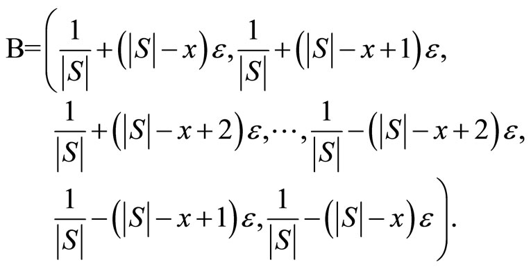 (4)
(4)
The idea is to make sure that if we add e to x number of probabilities, then we also subtract e from another x number of probabilities. The main goal is that each addition of e should be compensated by a subtraction of e so that we can keep the sum of probabilities equal to 1. The number of belief points that will be in the set B depends on the value of a density parameter a, where 0 < a < 1.
Algorithm 1 shows the algorithm that we have used to generate belief points. In this algorithm, the array Bel is initialized with the initial belief point b0, as defined above, in all its indices. Line 1 determines the maximum and minimum boundary of e which are 1/|S| and 0 respectively. In line 1, a is added to e on each iteration until it reaches the maximum boundary. Lines 2 through 5 specify the range of indices where values will be increased or reduced. On lines 9 to 12, we subtract e from the values in index k to l of the Bel array which has initial belief in each iteration. After computing new belief values in line 10 we add them to our belief set B. On lines 13 to 16, we add e to the values in index i to j and insert these values to B as well. If the number of subtractions by e exceeds the number of additions by e, then we fix the difference by adding the value of the number of excess times e to the final index in lines 17 to 19. We maintain the sum of addition and subtraction between indices by variables increased Sum and reduce Sum in each iteration respecttively. Belief points are only generated once. The belief set remains constant through all iterations of the POMDP algorithm.
3.2. The Scan Line
A parameter β is used to chose the belief points in B that will participate in the scanning procedure. The value of β indicates how many belief points from the current one will be skipped as the scan is performed.
After the set of belief points B is generated, as shown in Figure 1 for 2 states problem, we take a belief b ∈ B, calculate the expected rewards associated with b, find the maximum, and record the corresponding vector (i.e. value function) that is associated with the maximum reward. This procedure goes on until we have exhausted all the belief points in B or the number of remaining belief points is less than the value of β or the set of value functions associated with the maximum rewards is equal to the set of value functions.
4. Recursive Point Filter (RPF)
In RPF, we begin by pruning completely dominated vectors, which means that we must first eliminate any vector Vi that satisfies Vi < Vj ∀b ∈ β and j ≠ i. This property can hold for collinear planes or for planes that are dominated component-wise for all states. We can notice that after eliminating these vectors, we are only left with intersecting planes.
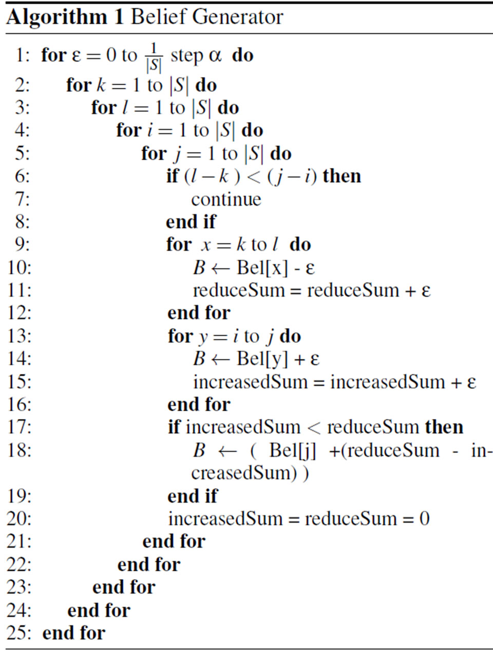
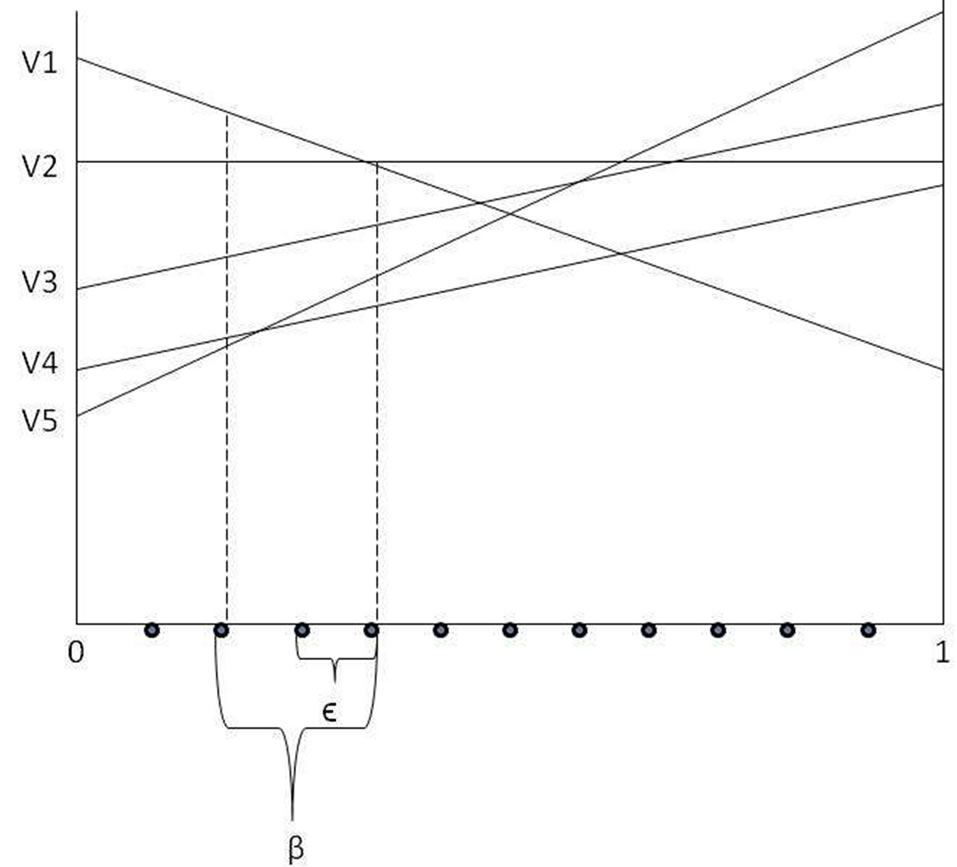
Figure 1. 2D vectors in two states belief space.
4.1. RPF in a 2-States Belief Space
Since pruning eliminates the set of vectors which are not part of the final solution, it is an important part to make most of the POMDP solvers faster.
In each recursion of RPF (Algorithm 2), it gets two real numbers {InterStart, InterEnd} as the inputs and returns the dominated vectors list {PrunedList}. InterStart, InterEnd are the starting and ending points in the interval of one dimensional belief space. In the next step, it calculates MidPnt as the middle point between InterStart, InterEnd. It is obvious that initially InterStart, InterEnd are set to 0 and 1 respectively. If |InterStart-InterEnd| < δ ,δ is a positive parameter set before beginning of the recursion; it exits before entering into the main loop of the algorithm. Otherwise, it identifies dominated vectors within given belief intervals :{InterStart to MidPnt} and {MidPnt to InterEnd}. We call the dominated vector with belief value of MidPnt as Vmid, Inter-Start as Vsrt, InterEnd as Vend respectively (lines 4 - 6). In the next part of the algorithm, it compares Vmid with Vsrt; if they are from the same vectors, it adds Vsrt into PrunedList (line 14), and the witness region is extended by adding the boundary of dominated vectors. In the next recursion it gets new intervals InterStart, (MidPnt + InterStart)/2 as new arguments for 2 the RPF algorithm (line 12). In this way, it recognizes upper surface vectors from InterStart to MidPnt. We use the same approach for (MidPnt + InterStart)/2, InterEnd (lines 16 - 20), recursively to cover remaining part of the belief space interval.
Figure 2 shows an incomplete execution of the RPF for six vectors after four recursive calls. It recognizes upper surface vectors from belief points between 0 to 0.5 (where δ ← 0.05 is set before the execution) for a 2- states problem. When RPF is terminated, a list of identified dominated vectors will be returned by the PrunedList .
4.2. RPF in Higher Dimensions
In the 2D representation, a horizontal axis is the belief space while a vertical axis is showing the values of each vector over the belief space. Since most of the POMDP problems have more than two states; it makes value function to be represented as a set of hyperplanes instead of 2D vectors. In other words, a POMDP problem with |S| number of states makes (|S|-1) dimensional hyperplanes for representing in the belief space. A POMDP policy is then a set of labelled vectors that are the coeffi-
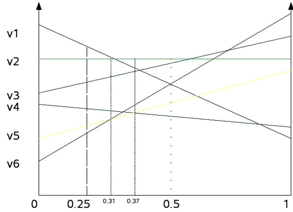
Figure 2. Incomplete execution of RPF over a 2-states belief space (δ = 0.05).
cient of the linear segments that make up the value function. The dominated vector at each corner of the belief space is obviously dominant over some region [13]. As mentioned since RPF receives 2D vectors as the input arguments; the filter algorithm projects every hyperplane into 2D planes and then passes 2D vectors set to RPF algorithm. It sets zero to every component of hyperplane equations except ones that are in the 2D plane equations. Hence, the projections of hyperplanes are 2D vectors, therefore a set of 2D vectors in each plane now can be passed to RPF for filtering. There are  possible 2D planes where |S| is the number of states. As shown in Figure 3" target="_self"> Figure 3, each 3D vector represents value function of
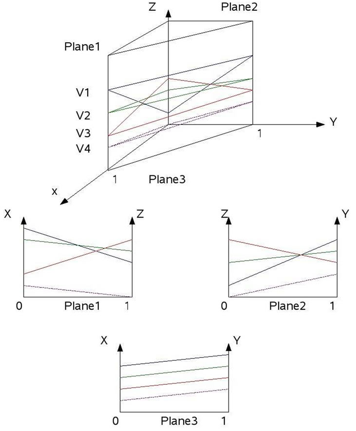

Figure 3. Value function is shown as a plane in a 3-states POMDP problem.
one action.As indicated, after each projection, RPF gets a set of 2D vector equations and starts filtering. In filtering process, in each plane, if any of the 2D vectors is part of a 2D upper surface, its corresponding hyperplane index is labelled as dominated vector and its index will add to final pruned vectors list.
5. Experimental Results
5.1. Empirical Results
Asymptotic analysis provides useful information about the complexity of an algorithm, but we also need to provide an intuition about how well an algorithm works in practice on a set of problems. Another disadvantage of Asymptotic analysis is that it does not consider constant factors and operations required outside the programs. To address these problems, we have run SCF, LP, RFP on the same machine which had 1.6 GHz AMD Athlon Processor with 2 Gb RAM on a set of the benchmark problems from the POMDP literature. These problems are obtained from Cassandra’s Online repository [14].
For each problem and method we report the following:
1) size of the final value function (|V|);
2) CPU time until convergence;
3) resulting ADR;
The number of states, actions and observations are represented by S, A and Z.
As with most exact methods, a set of linear actionvalue functions are stored as vectors representing the policy. In each iteration of running algorithm, the current policy is transformed into a new set of vectors which are then filtered in three stages. As mentioned in chapter 2, each stage produces a unique minimum size set of vectors. This cycle is repeated until the value function converges to a stable set of vectors. The difference between two successive vector sets make an error bound. The algorithms are considered to have converged when the error bound is less than a threshold of convergence (For example, The ε parameter in LP algorithm). However, a final set of vectors after convergence does not guarantee an optimal solution until the performance of the policy is considered under a simulator of the POMDP model. Changing ε to a higher value would lead to a non-optimal solution, and on the other hand if it is set to a lower value; it may loop between two sets of vectors because of numerical instability of solvers. Although 0.02 may not be the absolute minimum value for ε, but we believe that it is small enough to provide the precision for evaluating policies in the simulator.
Table 1 shows parameter values of α, β, ε and δ for each POMDP problem in the SCF,LP and RPF algorithms. Each of these parameters are initialized to base value depending on the quality of the final POMDP solution and the characteristic of each POMDP model. As stated above, dynamic programming update is divided into three phases in all POMDP solvers. Therefore, we have the same structure of Incremental Pruning in our solvers that are different in their filtering algorithms.
We have evaluated based on their average CPU time spent to solve each problem. All POMDP solvers were allowed to run until they converged to a solution or they exceed a 24 hours maximum running time. Previous research on the POMDP solvers [9], has shown that POMDP exact solvers for the classical test-bed problems either find a solution before 12 hours or they can-not converge. Our hypothesis is, because of the numerical instability they may oscillate between two successive iterations.
Table 2 summarizes the experiments for all three POMDP solvers. In this table RPF was compared to linear programming filtering (LP) and scan line filtering (SCF) techniques. An x on the table means that the problem did not converge under the maximum time limit set to perform the experiment; therefore we are unable to indicate how many vectors (i.e. Value functions) form the final solution. The Vector column on the table indicates how many vectors form the final solution and the Time column shows average CPU time in second over 32 executions. Having higher number of vectors in the final solution and less convergence time are two major positive factors that are considered in our evaluation. We define the term better in our evaluation when a POMDP solver can find solution of a problem in lesser time with more final value functions (|V|) than others.
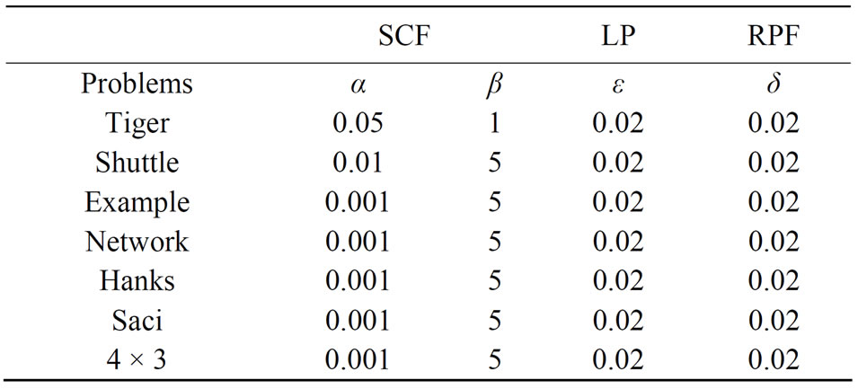
Table 1. α, β, ε and δ parameters for the SCF, LP and RPF algorithms.
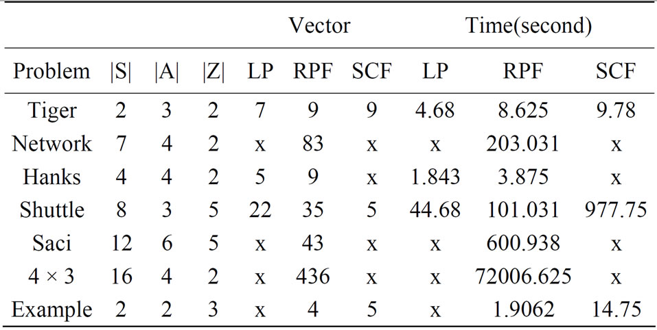
Table 2. Experiment I descriptions and results presented as the arithmetic mean of 32 run-times.
From the Table 2 we can see that RPF found solution on POMDP problems Network, Scai, 4 × 3 while SCF and LP were not able to converge to a solution before 24 hour limit. In the term of size of the final value function (|V|), RFP had more vectors than both SCF and LP in the Shuttle, and more than LP in Hanks and the Tiger problems. It also shows RPF is faster than SCF in Tiger, Shuttle and the Example but slower than LP approach in the problems that LP solved: Tiger, Hanks and Shuttle. RPF is better than the others in POMDP problems Network, Scai and 4 × 3.
5.2. Parameter Testing of SCF Filter with the Tiger Problem
Our SCF filter has two adjustable parameters, α and β. α is the density parameter and is also the value used to check whether or not two rewards are significantly different. The value of β indicates how many belief points will be skipped at each iteration of the scan. In the Tiger problem, each value of α corresponds to a specific number as illustrated by Table 3.
Here, our goal was to find the values for α and β under which our approach would be faster on solving the tiger problem. Table 4 expresses the results of this experiment, which was performed on a 2 Ghz Intel Core 2 processor.
From Table 4, we can see that setting α = 0.1 and β = 1 resulted in shorter run time than any other setting. For the tiger problem, our approach seems to perform fastest by considering 67 belief points in total.
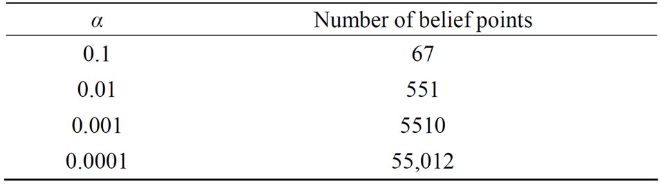
Table 3. Relation between α and number of belief points in tiger problem.

Table 4. Varying α and β in order to determine the best setting to solve the tiger problem.
5.3. Simulation
One way to evaluate the quality of policy is to run it under simulator and observe accumulated average of the discounted reward that agent received over several trials. A POMDP policy is evaluated by its expected discounted reward over all possible policy rollouts. Since the exact computation of this expectation is typically intractable, we take a sampling approach, where we simulate interacttions of an agent following the policy with the environment. A sequence of interactions, starting from b0, is called a trial. To calculate ADR, successive polices are tested and rewards are discounted, added and averaged accordingly. Each test starts from an arbitrary belief state with a given policy, Discounted reward is added for each step until the maximum steps limit is reached. The test is repeated for the number of trials. Steps are added among all the trials. The ADR is represented in the form of (mean ± confidence interval) among all tested policies. In our implementation of ADR, confidential interval is 95%
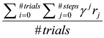 (5)
(5)
We computed the expected reward of each such trial, and averaged it over a set of trials, to compute an estimation of the expected discounted reward.
In this experiment, we have computed ADR for a subset of POMDP problems where the RPF algorithm and either LPF or SCF techniques have solutions. Since ADR values are noisy for the less number of trials, we have tested different number of trials starting with 500. After several tries, we saw that the difference between ADR means with 2000 trials and 2500 are small enough to chose 2000 as the final number of trials in our experiment. We tested such policies in the simulator with 500 steps for each POMDP problem over 2000 trials as shown in Table 5.
In general, RPF has the near close ADR values to other approaches. This implies RPF policy has a performance similar to SCF and LP for the set of problems we chose. Although LP is the winner in term of the ADR for the Tiger, but it has smaller ADR mean value for the rest of the problems than RPF. One hypothesis is size of |V| in LP policy in Table 2 for these problems is smaller than RFP; and it also shows that the value of computed ADR
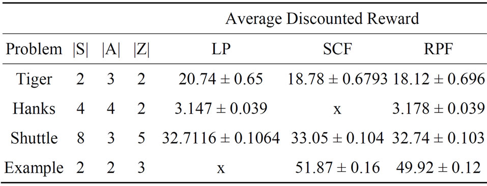
Table 5. Experiment II: average discounted reward.
mean under a policy is proportional to the size of the final value function (|V|). However, the policies of SCF in the Shuttle and LP in the Tiger problem are two exceptions that with less (|V|) we have observed nearly same or better ADR mean values than with higher (|V|). We believe that it may come from characteristics of the POMDP model. Therefore, since these values are nearly close to each other further experiments need to be done to prove our guesses.
6. Conclusions
6.1. Discussion
We considered two new filtering techniques, called Recursive Point Filter (RPF) and Scan Line Filter (SCF for Incremental Pruning (IP) POMDP solver to introduce an alternative method for Linear Programming (LP) filter. As suggested in the original work on Incremental Pruning technique, filtering takes place in three stages of an updating process, we have followed the same structure in our implementation to have a fair evaluation with previous approaches. RPF identifies vectors with maximum - values in each witness region known as dominated vectors. The dominating vectors at each of these points then become a part of the upper surface. We have shown that a highquality POMDP policy can be found in the less time in some cases. Furthermore, RPF had solutions for several POMDP problems that LP and SCF were not able to converge in 24 hours. As discussed in the paper, the quality of POMDP solutions of LP approach depends on the numerical stability of LP solver. Also, LP based filter requires LP libraries, which can be expensive, especially the powerful ones. Because of these reasons, we proposed the idea of filtering vectors as a graphical operator in POMDP solver. In each iteration of the algorithm, vectors that are not part of the uppersurface would be eliminated. SCF and RPF use the same concept but with different algorithmic ways. Although SCF had better performance in some POMDP problems, but it is dependent on the parameters (α, β) for each POMDP problem. It means that SCF parameters have direct effect on the quality of solution and convergence time for each POMDP problem. RPF was superior on several POMDP problems while SCF was not able to converge to solutions before 24 hours or had lesser number of vectors in the final solutions with some values for α, β.
We also included Average Discounted Reward in our evaluation for a sub-set of POMDP problems where the RPF, LP or SCF techniques have solutions. We tested such policies in the simulator with 500 steps for the POMDP problems over 2000 trials. The promising result is, RPF and SCF have a closer ADR mean value than other approaches. This implies RPF and SCF policy have a performance similar to LP for the set of problems we chose.
Although RPF worked better in the small classical POMDP problems, but it has poor performance on bigger sized POMDP problems such as: Mini-hall, Hallway, Mit [14]. Because of this reason and also our paper consideration on smaller size problems, we believe that for large POMDP problems like those discussed above, approximate techniques would be a better option to choose. If the complexity of a POMDP problem is close to our set of evaluation, then LP, with the condition that the size is close enough to the Tiger problem, is suggested. If LP is not available, or is expensive and the size of the POMDP problem is not close to the ones that LP was winner in, then RPF and SCF are recommended. Although RPF was superior to SCF in some cases but it does not strongly show that with all values of α, β this condition would be held. However, SCF Parameter Tuning is essential for more consideration of finding solutions in POMDP problems where it has poor performance.
6.2. Future Works
Since SCF parameters have important rules either in finding POMDP solution or increasing the size of the final Value function (|V|), we will improve SCF with a dynamic setting parameters approach and compare results with RFP on the sub-set of the POMDP problems where RPF was a winner.
Our initial objective in this research was to present an alternative solver to evaluate approximate solutions on POMDP problems with small number of states. We are going to extend our implementation to use parallel processing over CPU nodes to test RPF on larger POMDP problems like Hallway to evaluate solutions of approximate techniques. We also intend to log the number of pruned vectors in each iteration of the algorithms for more consideration on how well each algorithm performs pruning on average after a large number of iterations and when the convergence threshold changes.
REFERENCES
- G. E. Monahan, “A Survey of Partially Observable Markov Decision Processes,” Management Science, Vol. 28, No. 1, 1982, pp. 1-16. doi:10.1287/mnsc.28.1.1
- R. D. Smallwood and E. J. Sondik, “The Optimal Control of Partially Observable Markov Processes over a Finite Horizon,” Operations Research, Vol. 21, 1973, pp. 1071- 1088. doi:10.1287/opre.21.5.1071
- P. E. Caines, “Linear Stochastic Systems,” John Wiley, New York, 1988.
- M. T. J. Spaan, “Cooperative Active Perception Using POMDPs,” AAAI 2008 Workshop on Advancements in POMDP Solvers, 2008.
- J. Goldsmith and M. Mundhenk, “Complexity Issues in Markov Decision Processes,” Proceedings of the IEEE Conference on Computational Complexity, New York, 1998.
- J. Pineau, G. Gordon and S. Thrun, “Point-Based Value Iteration: An Anytime Algorithm for POMDPs,” Proceedings of the International Joint Conference on Artificial Intelligence, Acapulco, 2003.
- T. Smith and R. G. Simmons, “Heuristic Search Value Iteration for POMDPs,” Proceedings of the International Conference on Uncertainty in Artificial Intelligence, Banff, 2004.
- M. T. J. Spaan and N. Vlassis, “Randomized Point-Based Value Iteration for POMDPs,” Journal of Artificial Intelligence Research, Vol. 24, 2005, pp. 195-120.
- A. Cassandra, M. L. Littman and N. L. Zhang, “Incremental Pruning: A Simple, Fast, Exact Algorithm for Partially Observable Markov Decision Processes,” Proceedings of the 13th Annual Conference on Uncertainty in Artificial Intelligence, Brown, 1997.
- R. Moore, “A Formal Theory of Knowledge and Action,” In: J. Hobbs and R. Moore, Eds., Formal Theories of the Commonsense World, Norwood, 1985, pp. 319-358.
- A. R. Cassandra, L. P. Kaelbling and M. L. Littman, “Acting Optimally in Partially Observable Stochastic Domains,” Proceedings of the 12th National Conference on Artificial Intelligence, Seattle, 1994.
- M. Littman, A. Cassandra and K. L. P, “Efficient Dynamic-Programming Updates in Partially Observable Markov Decision Process,” Brown University, Providence, 1996.
- L. D. Pyeatt and A. E. Howe, “A Parallel Algorithm for POMDP Solution,” Proceedings of the 5th European Conference on Planning, Durham, 1999, pp. 73-83.
- A. R. Cassandra, “Exact and Approximate Algorithms for Partially Observable Markov Decision Process,” PhD Thesis, Brown University, Brown, 1998.