Open Journal of Soil Science
Vol.05 No.06(2015), Article ID:57030,11 pages
10.4236/ojss.2015.56012
The Effect of the Geomorphologic Type as Surrogate to the Time Factor on Digital Soil Mapping
Huixia Chai1, Sheng Rao1, Reibo Wang2, Jing Liu3, Qi Huang1, Xuejie Mou1
1Chinese Academy for Environmental Planning, MEP, Beijing, China
2State Key Laboratory of Resources and Environmental Information System, Institute of Geographical Sciences and Natural Resources Research, CAS, Beijing, China
3Department of Geography, University of Wisconsin-Madison, Madison, USA
Email: chaihx@caep.org.cn
Copyright © 2015 by authors and Scientific Research Publishing Inc.
This work is licensed under the Creative Commons Attribution International License (CC BY).
http://creativecommons.org/licenses/by/4.0/


Received 7 May 2015; accepted 7 June 2015; published 10 June 2015
ABSTRACT
Many environmental variables are frequently used to predict values of soil in locations where they are not measured. Digital soil mapping (DSM) has a long-standing convention to describe soils as a function of climate, organisms, topography, parent material, time and space. It is obvious that terrain, climate, parent material and organisms are used frequently in the prediction of soil properties while time and space factors are rarely used. Time is the indirect factor for the formation and development of soil. Moreover, it is very useful to explicit and implicit estimates of soil age for DSM. However, it is often difficult to obtain time factor. In the absence of explicit soil age data, geomorphologic data are commonly related to soil relative age. Consequently, this study adopts the geomorphologic types (genesis type of geomorphology) as surrogate to the time factor and analyzes its effect on DSM. To examine this idea, we selected the Ili region of northwestern China as the study area. This paper uses geomorphologic data from a new digital geomorphology map as the implicit soil age in predictive soil mapping. For this study, Soil-landscape inference model (SoLIM) was used to predict soil properties based on the individual representation of each sample. This model applies the terrain (topography), climate, parent material (geology) and time (geomorphologic type) to predict soil values in the study area where they are not measured. And the independent sample validation method was used to estimate the precision of results. The validation result shows that the use of geomorphologic data as surrogate to the time factor in the individual representation leads to a considerable and significant increase in the accuracy of results. In other words, implicit estimates of soil age by genesis type of geomorphology are very useful for DSM. This increase was due to the high purity of the geomorphologic data. This means that the geomorphologic variable, if used, can improve the quality of DSM. Predicted value through the proposed approach comes closer to the real value.
Keywords:
Geomorphologic Type, Environmental Variables, Digital Soil Mapping, Soil-Landscape Inference Model (SoLIM), Individual Validation

1. Introduction
Digital soil mapping (DSM) is a technology and method to describe the spatial distribution information of soil with a grid format on the basis of field samples and/or auxiliary data, such as soil environmental factors and other soil properties [1] . DSM has a long-standing convention to describe soils as an equation of climate, organisms, topography, parent material, and time [2] [3] . McBratney et al. [4] put forward a so-called “scorpan model” as a spatial predicted model of soil properties based on the environmental variables of climate, organisms, topography, parent material, time and space. Those variables, if their information is available for the location, are frequently used to predict values of soil in locations where they are not measured [5] - [9] . Therefore, these factors should consider into the methods or models of predicted soil properties, at least in theory. But in practice it is hard to do because it is too difficult to get or measure some environmental factors like time.
Studies use various approaches to predict soil properties by single-variable and multi-variable statistics [10] - [12] , geostatistical [13] - [15] and hybrid methods [16] [17] , and process-based models that relate soils to environmental covariates consider spatial and temporal dimensions [1] [4] [18] . Recently, most studies adopt the synthetic analysis and comprehensive applications of more environmental variables to predict the soil properties or the spatial distribution of soil [19] - [22] . However, it is obvious that terrain, climate, parent material (geology) and organisms (vegetation) are used frequently in the prediction of soil properties while time and space factors are rarely used.
Actually, it is very necessary to get the time factor into DSM. Time is the indirect factor for the formation and development of soil because it is a way to embody the effect of climate, organisms, topography, and parent material on the soil formation through time [3] . Explicit and implicit estimates of soil age are very useful environmental covariants for DSM, but are often difficult to obtain [12] . The temporal information of soil formation is unavailable, or not widely available, especially the absolute time, although some studies use the 14C detection or fossil analysis to obtain the soil age of sample points [23] [24] . Moonjun et al. [25] tried to find a correlation between the observed data (in the sample areas) and the environmental characteristics derived from the DEM, and they distinguish three relative soil ages: old (Ultisols and Oxisols), mature (Alfisols), and young (Inceptisols and Entisols). Noller [26] reviews various approaches to add geochronology in DSM and obtains the improved prediction of soil on the landscape in addition to several implicit age covariates, including custom thematic maps of lithology and geologic age. Therefore, it is important to get the time factor into DSM. Furthermore, how to accurately get the temporal information of soil formation is always a problem in the whole study area only based on few observed data of field samples. Generally, in the absence of explicit soil age data, implicit topographic data representing landforms that are commonly related to soil relative age and remotely sensed spectral data that focus on surface spectral characteristics represent surface or soil age [12] .
Consequently, the purpose of this study is to analyze the effect of the genesis types of geomorphology as surrogate to the time factor on DSM. In other words, this study adopts the geomorphologic types as the relative time in the process of DSM. To analyze the effect of geomorphologic types on DSM, this study uses the SoLIM (a professional software for DSM) to predict soil organic matter (%) of the top layer in locations where they are unknown.
2. Basic Idea
2.1. Theory
Geomorphology is one of the predominant factors determining the features of the earth’s surface and an important symbol and dominant factor of regional differentiation. It (geomorphology) directly influences and even decides the spatial distribution and transformation of hydrology, climate, soil, and other ecological and environmental factors [27] . Since in 1980, Knott et al. [28] had been analyze and find that the geomorphologic mapping boundaries are coincident with soil material boundaries, which implies a correlation between soil material and geomorphology to some degree. Geomorphologic processes, both erosional and depositional, create distinctive landforms which have a great influence on soil types and soil distribution [29] . The soil condition is different in places with various geomorphologic types due to the forming reason of geomorphology, as well as in different parts of geomorphology. The forming reason of geomorphology means that it will appear in some dominant geomorphologic processes, and produce characteristic landforms in particular climatic conditions [30] . Bacon et al. [31] point that systematic relationships exist between landscapes position (terrain conditions of desert landform) and soil formation processes. In their study, the assignment of relative age classes to each landform or geomorphic surface map unit was based on crosscutting relations, surface morphology and roughness, and topographic relief observable on the multispectral imagery. Moreover, Stum et al. [32] use landform surface age as the implicit soil age in predictive soil mapping by spatially modeling the shoreline of Pleistocene pluvial Lake Bonneville.
Therefore, we consider that the geomorphologic type could be used to approximate the time factor at the categorical level in soil formation processes. In other words, this study wants to take the geomorphologic type as surrogate to the time factor on DSM. The geomorphologic type here specifically means the genesis type of geomorphology. The genesis type is classified by the forming reason of geomorphology. It is a nominal variable and only represents the relative time.
2.2. Experiment Design
The process of DSM in this study was based on the Soil-landscape inference model (SoLIM). SoLIM is a new technology for soil mapping based on recent developments in Geographic Information Sciences (GIS), Artificial Intelligence, and Information Representation Theory. SoLIM was designed to overcome the limitations of existing soil survey methods and to improve the efficiency and accuracy of soil surveys [3] . Case studies have shown that SoLIM is more efficient and accurate than traditional soil survey methods, in that it generates a range of products which the traditional approaches couldn't provide, and it can be employed in a production mode of soil survey.
This study adds the geomorphologic type as surrogate to the relative time of soil and use the sampled-based approach under the SoLIM framework to examine the effect of including geomorphologic type. The environmental variables in this study (Table 1) including topography (Terrain, derive from DEM), climate, parent material (obtain from geology map) and time (relative time, using geomorphologic type as indicator).
This study describes two experiments to test the idea mentioned above. Each experiment has different environmental variables. The first group of environmental variables includes climate, parent material and topography. The second group includes climate, parent material, topography and geomorphology. Based on two groups of environmental variables, this paper presents two soil maps by the same research methods. Then we compare and analyze the precision between the two soil maps.
3. Method and Data
This section provided an introduction to study area, data and method in this study. By the way, readers can refer to literatures [3] [33] if you are interested in a comprehensive description of prediction method. Based on the knowledge of the relationship between soil and environment, this paper selected four environmental (Table 1) variables to describe environmental features. Climate data and geomorphic types collected by State Key Laboratory of Resource and Environmental Information System, IGSNRR, CAS. Parent material rasterized from Chinese Geology Map (1:1000,000). Seven topographic covariates (altitude (m), slope gradient (%), aspect, contour curvature, profile curvature, Plane curvature, Surface area ratio (SAR), Topographical wetness index (TWI)) were derived from DEM, which was downloaded from SRTM website.
3.1. Study Area
The study area of this research is the Ili region located between 42˚14'16''N and 44˚50'30''N, 80˚09'42''E and 84˚56'50''E, Xinjiang Uygur Autonomous Region, China (Figure 1). The Ili region is about

Figure 1. Study area.

Table 1. Environmental variables and their resolution.
from the general distribution pattern at certain locations. The amount of annual precipitation on the flat plain is about 140 -
The main parent materials are quartz sand, mica sand, red mudstones and alluvial loess or alluvial loess-like materials. Thanks to the variation of climate, terrain, vegetation and parent material conditions, soil types are relatively abundant on both vertical and horizontal distributions, mainly including chestnut soil, chernozem soil, forest soil, meadow soil, and Sierozem soil.
The basic geomorphology in the study area is composed of mountain landform and river-valley landforms. Geomorphologic types in the mountains at extremely high or high altitudes are mainly glacial and periglacial landforms. The lower part of the mountains is mainly fluvial landforms which formed by the erosion action of water and arid landforms which formed by a dry eroding effect. Alluvial plain, proluvial plain, and alluvial-pro- luvial plain are mainly distributed in the basin area. Fluvial landform is the dominant geomorphologic type in the plain landform area. In addition, the study area also has a small number of aeolian landform and loess landform.
3.2. Geomorphologic Data and Field Data
This paper collected all necessary data of study area, including climate data, SRTM-DEM, Geology Map, and the data of geomorphic types, to gain corresponding variables.
Geomorphology has a profound influence on the formation and development of soil by redistributing parent material, water, and heat. The geomorphologic type derives from the new 1:1,000,000 set of geomorphologic atlas of China. The digital geomorphologic database was created by visual interpretation from Landsat TM/ETM imageries, SRTM-DEM, and published geomorphologic maps, etc. [34] . The atlas was compiled and finished from the database, published by Science Press in 2009 [35] . The geomorphologic data include seven layers, i.e. basic morphology, genesis, sub-genesis, morphology, micro-morphology, slope and aspect, material composition and lithology. Here, we only use the genesis type of geomorphology to represents the relative time.
In addition, this paper also collected 107 soil sample data from the following sources: 1) National Native Soil Type Log (the Second National Soil Survey Office, 1995); 2) Field survey carried out by Dr. Ma Xingwang, Institute of Soil and Fertilizer, Xinjiang Academy of Agricultural Sciences; 3) Offered by Dr. Zhang Baiping and Dr. Zhang Hongqi, Institute of Geographical Sciences and Natural Resources Research, Chinese Academy of Sciences; 4) The book named Soil in Ili area, Xinjiang (1985).
3.3. Prediction Method and Computational Details
This paper adopts the independent sample validation method to estimate the performance of the predicted result. First, 75 of the 107 sampling were chosen to serve as sample points to predict soil properties. Then the other 32 soil samples serve as validation points to test the precision of DSM. Finally, estimate value of validation points would be extracted from the predicted result of 75 sample points through add validation points layer upon the result layer. This method can examine the precision of single point forecasting on two soil maps.
3.3.1. Environmental Variables
Climate data include annual-averaged precipitation, temperature and relative humidity, as well as the maximum and minimum of monthly-averaged precipitation, temperature and relative humidity within a year. These three variables have great influence on the decomposition and transformation of soil organic matter.
Topographical indexes include slope, aspect, profile curvature, plane curvature, surface area ratio and topographical wetness index. Topographical Wetness Index (TWI) is estimated according to a modified Multiple- Flow-Direction (MFD) algorithm [36] for calculating upslope drainage area. Surface Area Ratio (SAR), which represents the roughness within a mapping grid, is generated based on the algorithm developed by Jenness [37] . Other topographical variables are generated through ArcGIS. The content of surface soil organic matter often has a negative correlation to elevation [38] [39] . Slope, which represents the tilt degree of the local surface topography, has a direct relationship to the stability of soil, the drainage and gathering ability of surface water [39] [40] . Aspect affects the accumulation and decomposition of surface soil organic matter [41] . Curvature affects the spatial distribution of surface soil organic matter [42] . Surface Area Ratio (SAR) is used for distinguishing mountains and plains by terrain characteristics [43] . Topographical wetness index, which represents the drainage and gathering ability of soil, affects the content of surface soil organic matter [39] .
Parent material types are often used to describe the different characteristics of parent material [4] . They include quartz sand, mica sand, red mudstones, alluvial loess, alluvial loess-like materials, glacier and snow cover.
The geomorphologic type which mentioned in this paper is the genesis type of geomorphology. This study adopts the genesis type of geomorphology as surrogate to the time factor. In other words, the geomorphologic type should be regard as the relative time for DSM in this study. According to the forming reason of geomorphology, there are six geomorphologic types in the study area: loess landform, fluvial landform, Aeolian landform, arid landform, glacial landform, and periglacial landform.
3.3.2. Quantifying and Estimating Similarity
His study, as the resolution of climate, parent material and geomorphology information is approximate to the mapping grid, the single value method was adopted to represent climate and geological characteristics of each grid. As the resolution of topographical factors is refined, the probability distribution of each index was approximated to represent topographical characteristics of each grid. For estimating a smooth probability distribution curve, the Kernel Density Estimation (KDE) method has been adopted in this case study.
In this study GOWER distance was adopted to calculate climate similarity. GOWER distance measures the similarity between a given location (i, j) and a sample k on a series of environmental variables, standardized by the range of each variable [44] (Equation (1)):
 (1)
(1)
where m is the number of climate variables;  denotes the absolute difference on the v-th climate variable between location (i, j) and sample k;
  is the global value-range of the v-th climate variable. The value of overall climate similarity
 ![]() will be between 0 and 1.
will be between 0 and 1.
Parent material similarity and geomorphologic similarity were decided through Boolean function. If the parent material type and geomorphologic type at the location (i, j) are identical with sample point k, it means parent material similarity and geomorphologic similarity are equal to 1, conversely, parent material similarity and geomorphologic similarity equal 0.
Similarity on each topographical index is calculated through the Consistency Measure (CM) algorithm, and finally, the integrated topographical similarity for all topographical indexes was estimated by an average-ope- rator (Equation (2)).
![]() (2)
(2)
where ![]() denotes the topographical similarity between location (i, j) and sample k; m is the number of involved topographical indexes;
denotes the topographical similarity between location (i, j) and sample k; m is the number of involved topographical indexes; ![]() is the Consistency index of the probability density distribution function on the v-th topographical variable between location (i, j) and sample k.
is the Consistency index of the probability density distribution function on the v-th topographical variable between location (i, j) and sample k.
Based on the importance of each environmental variable which indicates spatial distribution of soil at different scales, this paper generates the similarity between location point and sample point through comprehensive analysis of climate similarity, parent material similarity, topographical similarity and similarity of geomorphologic type (Figure 2 and Figure 3).
Please note the similarities and differences between Figure 2 and Figure 3.
Bothe figures have three things in common. Firstly, C_similarity, Topo_similarity means climate similarity, topographical similarity separately. Secondly, weights of climate similarity and topographical similarity both are 0.5. Thirdly, climate similarity cut is 0.5.
Figure 2 and Figure 3 have one difference. In Figure 2, environmental variables include climate, parent material and topography. Figure 3 has one more environmental variable than Figure 2, environmental variables include climate, parent material, topography and geomorphologic type.
First, this paper examines the climate similarity between an unsampled location and a certain case (a climate- similarity-cut was set at 0.5 and has been adopted generally as we had no background information on deciding this threshold).
Then, we test the parent material similarity if the unsampled location was similar enough with the case on climate.
Third, this paper continue to examine the geomorphologic similarity if the parent material of the unsampled location is the same as the case (it means the parent material similarity is equal to 1).
Finally, the topographical similarity and climate similarity would be integrated to estimate the final similarity using the weighted-average method if the geomorphologic similarity is equal to 1 (it means the geomorphologic
![]()
Figure 2. P-function for integrating environmental similarity into case-simi- larity.
![]()
Figure 3. P-function for integrating environmental similarity into case-simi- larity.
type of the unsampled location is the same as the case).
Here, the weights of the topographical similarity and climate similarity should be assigned considering the relative importance between them. As we had no knowledge to decide which one is more important, we assigned 0.5 to both as the weights.
The estimation of the value of the targeted soil property is calculated with a weighted average method [3] :
![]() (3)
(3)
in which n’ is the number of the selected soil samples whose environmental similarity to the unvisited location (i, j) exceeds 1 minus the uncertainty threshold, ![]() is the environmental similarity of the unvisited location (i, j) to the soil type k in sample location k, and Vk is the value of the targeted soil property of soil sample location k.
is the environmental similarity of the unvisited location (i, j) to the soil type k in sample location k, and Vk is the value of the targeted soil property of soil sample location k.
4. Result and Discussion
4.1. Predicted and Discussion
Figure 4 shows soil organic matter (%) of the top layer predicted through the proposed approaches. The gray area with “No-Data” is the grid which cannot be represented by current samples. Figure 4(b) is the result on the basis of three environmental variables: climate, parent material and topography. Figure 4(b) is the result on the basis of four environmental variables: climate, parent material, topography and geomorphology.
The result shows that estimated value through the proposed approaches is closer to the real value than to the average value. In other words, the proposed approach in this paper is valid. These graphs (Figure 4) show that the spatial distribution of soil organic matter content has little difference between the two results. It can help avoid wasting time and energy if the geomorphologic type is added as surrogate to the time factor in the process
![]() (a)
(a)![]() (b)
(b)
Figure 4. Soil organic matter (%) of top layer predicted though the proposed approach. (a) Without geomorphology; (b) With geomorphology.
of DSM. This means it will improve work efficiency.
4.2. Validation and Discussion
Generally, the mean/mean-bias error (ME or MBE), the mean absolute error (MAE), and the root mean squared error (RMSE) are used to test the error statistic. In this paper, the deviations of validation results are summarize by RMSE and MAE.
The root mean squared error (RMSE) provide a measure of estimation error that was more sensitive to outliers than the MAE
 (3)
(3)
where the generated predicted value represent by , the true observation value represent by
 . So, predicted error at each sample point describe by
 .
.
The mean absolute error (MAE) reflects the absolute error of the estimates. It is expressed as follows
 (4)
(4)
For 32 validation points, only 20 points have effective values, the rest of the validation points are located in the place where without predicted value. So, this paper just adopts the predicted values of these 20 points to calculate RMSE and MAE.
Table 2 shows the validation results of two experiments within different environmental variables. Table 2 indicates that the root mean squared error (RMSE) and the mean absolute error (MAE) are lower significantly after the data layer of geomorphologic type is added. It explains that the geomorphology variable can improve the accuracy of the predicted results in soil organic matter mapping. The values of RMSE and MAE with geomorphology are less than that without geomorphology. The value of RMSE without geomorphology is three times as big as the values of RMSE with geomorphology. This result indicating that the accuracy of predicted results with geomorphologic type is higher than one without geomorphologic type.
According to the validation results, most predicted values with geomorphology of validation samples are closer to real values than predicted values without geomorphology (Figure 5 and Figure 6). It can veritably reflect the soil properties if the geomorphologic type is added as the relative time. After adding the geomorphology variable, the accuracy rate of predicted values have been increased by an average of 34%. In other words, the predicted result with geomorphology is much better than the predicted result without geomorphology.
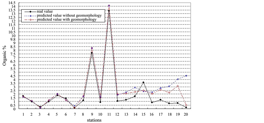
Figure 5. Comparative analysis of the real values, predicted values without geomor- phology and with geomorphology.
Table 2. Validation results.

Figure 6. Comparative residual of the predicted values without geomorphology and the predicted values with geomorphology.
5. Conclusions
There is no universal soil equation or digital soil prediction model that fits all regions and purposes [11] . Hence, the soil prediction at different scales (local, national and global scales) needs to build various equations and models respectively. This study adopts the geomorphologic type to represent the relative time of soil age and estimate the effect of the geomorphologic type on the predicted precision of DSM. We consider genesis type of geomorphology as surrogate to the time factor and predict soil organic matter through the SoLIM. This study tries to analyze the effect of the geomorphologic types as surrogate to the time factor on DSM by the case study.
The result shows that using the geomorphologic type as surrogate to the time factor can improve the result quality of DSM. The genesis type of geomorphology results in the estimated value closer to the real value. Validation with a probability sample shows that use of geomorphology data as the relative time factor leads to a considerable and significant increase of accuracy. In other words, implicit estimates of soil age by genesis type of geomorphology are very useful for DSM. There are 75% predicted values having been increased. This increase in accuracy is due to the high precision of the existing geomorphology data.
In addition, with such a limited sample-set and such complex natural conditions, it is probably not reasonable to adopt any of the current interpolation method to predict soil property values over the entire study area. That’s why there are many empty values in Figure 4. Therefore, in order to further test the degree of influence of the geomorphology variable on the precision of DSM, more samples are needed. This will be the author’s next step, a quantitative description of the degree of influences of the geomorphology variable on the precision of DSM.
Acknowledgements
The authors would like to thank anonymous reviewers for very helpful suggestions that were used to improve the manuscript.
References
- McBratney, A.B., Odeh, I.O.A., Biship, T., Dunbar, M.S. and Shatar, T.M. (2000) An Overview of Pedometric Techniques for Use in Soil Survey. Geoderma, 97, 293-327. http://dx.doi.org/10.1016/S0016-7061(00)00043-4
- Jenny, H. (1941) Factors of Soil Formation: A System of Quantitative Pedology. Dover Publications, New York, 281 p. http://books.google.com/books?id=p94TjEnzCTcC&dq=Factors+of+Soil+Formation:+A+System+of+Quantitative+Pedology&printsec=frontcover&source=bn&hl=en&ei=XfXZS_udG5OINtr74Ug&sa=X&oi=book_result&ct=result&resnum=4&ved=0CBkQ6AEwAw#v=onepage&q&f=false
- Zhu, A.X., Li, B.L. and Pei, T. (2008) Model and Method of Detail Digital Soil Survey. Science Press, Beijing. (In Chinese)
- McBratney, A.B., Mendonça Santos, M. and Minasny, B. (2003) On Digital Soil Mapping. Geoderma, 117, 3-52. http://dx.doi.org/10.1016/S0016-7061(03)00223-4
- Zhu, H.J. and He, Y.G. (1991) Soil Geography. Higher Education Press, Beijing. (In Chinese)
- Wu, G.H., Tian, L.S., Hu, S.X. and Wang, N.A. (2000) Natural Geography. Higher Education Press, Beijing. (In Chinese)
- Florinsky, I.V., Eilers, R.G., Manning, G.R. and Fuller, L.G. (2002) Prediction of Soil Properties by Digital Terrain Modelling. Environmental Modelling & Software, 17, 295-311. http://dx.doi.org/10.1016/S1364-8152(01)00067-6
- Li, T.J., Zhao, Y., Zhang, K.L., Zheng, Y.S. and Wang, Y. (2004) Soil Geography. Higher Education Press, Beijing. (In Chinese)
- Mendonça-Santos, M.L., Dart, R.O., Santos, H.G., Coelho, M.R., Berbara, R.L.L. and Lumbreras, J.F. (2010) Digital Soil Mapping of Topsoil Organic Carbon Content of Rio de Janeiro State, Brazil. In: Boettinger, J.L., Howell, D.W., Moore, A.C., Hartemink, A.E. and Kienast-Brown, S., Eds., Digital Soil Mapping, Springer Science + Business Media B.V., New York, 255-266. http://dx.doi.org/10.1007/978-90-481-8863-5_21
- Moore, I.D., Gessler, P.E., Nielsen, G.A. and Peterson, G.A. (1993) Soil Attributes Prediction Using Terrain Analysis. Soil Science Society of America Journal, 57, 443-452. http://dx.doi.org/10.2136/sssaj1993.03615995005700020026x
- Grunwald, S. (2009) Multi-Criteria Characterization of Recent Digital Soil Mapping and Modeling Approaches. Geoderma, 152, 195-207. http://dx.doi.org/10.1016/j.geoderma.2009.06.003
- Boettinger, J.L. (2010) Environmental Covariates for Digital Soil Mapping in the Western USA. In: Boettinger, J.L., Howell, D.W., Moore, A.C., Hartemink, A.E. and Kienast-Brown, S., Eds., Digital Soil Mapping, Springer Science + Business Media B.V., New York, 17-27. http://dx.doi.org/10.1007/978-90-481-8863-5_2
- Odeh, I.O.A., McBratney, A.B. and Chittleborough, D.J. (1992) Fuzzy-c-Means and Kriging for Mapping Soil as a Continuous System. Soil Science Society of America Journal, 56, 1848-1854. http://dx.doi.org/10.2136/sssaj1992.03615995005600060033x
- Bourgault, G., Journel, A.G., Rhoades, J.D., Corwin, D.L. and Lesch, S.M. (1997) Geostatistical Analysis of a Soil Data Set. Advances in Agronomy, 58, 241-292.
- Hendricks Frassen, H.J.W.M., van Eijnsbergen, A.C. and Stien, A. (1997) Use of Spatial Prediction Techniques and Fuzzy Classification for Mapping Soil Pollutants. Geoderma, 77, 243-262. http://dx.doi.org/10.1016/S0016-7061(97)00024-4
- Odeh, I.O.A., McBratney, A.B. and Chittleborough, D.J. (1995) Further Results on Prediction of Soil Properties from Terrain Attributes: Heterotopic Cokriging and Regression-Kriging. Journal of Geoderma, 67, 215-225. http://dx.doi.org/10.1016/0016-7061(95)00007-B
- Odeh, I.O.A. and McBratney, A.B. (1998) Using NOAA Advanced Very High Resolution Radiometric Imageries for Regional Soil Inventory. Proceedings of the 16th World Congress of Soil Science, Montpellier, 20-26 August 1998. http://natres.psu.ac.th/Link/SoilCongress/bdd/symp17/498-r.pdf
- Grunwald, S. (2010) Current State of Digital Soil Mapping and What Is Next. In: Boettinger, J.L., Howell, D.W., Moore, A.C., Hartemink, A.E. and Kienast-Brown, S., Eds., Digital Soil Mapping, Springer Science + Business Media B.V., New York, 3-12. http://dx.doi.org/10.1007/978-90-481-8863-5_1
- Boettinger, J.L., Ramsey, R.D., Bodily, J.M., Cole, N.J., Kienast-Brown, S., Nield, S.J., Saunders, A.M. and Stum, A.K. (2008) Landsat Spectral Data for Digital Soil Mapping. In: Hartemink, A.E., McBratney, A.B. and MendonÇa-Santos, M.L., Eds., Digital Soil Mapping with Limited Data, Springer Science + Business Media B.V., New York, 193-202.
- Gonzalez, J.P., Jarvis, A., Cook, S.E., Oberthür, T., Rincon-Romero, M., Bagnell, J.A. and Dias, M.B. (2008) Digital Soil Mapping of Soil Properties in Honduras Using Readily Available Biophysical Datasets and Gaussian Processes. In: Hartemink, A.E., McBratney, A.B. and MendonÇa-Santos, M.L., Eds., Digital Soil Mapping with Limited Data, Springer Science + Business Media B.V., New York, 367-380.
- Roecker, S.M., Howell, D.W., Haydu-Houdeshell, C.A. and Blinn, C. (2010) A Qualitative Comparison of Conventional Soil Survey and Digital Soil Mapping Approaches. In: Boettinger, J.L., Howell, D.W., Moore, A.C., Hartemink, A.E. and Kienast-Brown, S., Eds., Digital Soil Mapping, Springer Science + Business Media B.V., New York, 369-384. http://dx.doi.org/10.1007/978-90-481-8863-5_29
- Wiesmeier, M., Barthold, F., Blank, B. and Kögel-Knabner, I. (2011) Digital Mapping of Soil Organic Matter Stocks Using Random Forest Modeling in a Semi-Arid Steppe Ecosystem. Plant and Soil, 340, 7-24. http://dx.doi.org/10.1007/s11104-010-0425-z
- Wysocki, D.A., Schoeneberger, P.J. and LaGarry, H.E. (2000) Geomorphology of Soil Landscapes. In: Sumner, M.E., Ed., Handbook of Soil Science, CRC Press, New York, E5-E39.
- Yang, M.S., Zhang, H.C., Ding, H., Lei, G.L., Fan, H.F., Chang, F.Q., Li, B., Zhang, W.X., Niu, J. and Chen, Y. (2005) 14C Dating of Paleosol and Animal Remains in Loess Deposit: A Comparative Study. Journal of China University of Geosciences, 30, 589-596.
- Moonjun, R., Farshad, A., Shrestha, D.P. and Vaiphasa, C. (2010) Artificial Neural Network and Decision Tree in Predictive Soil Mapping of Hoi Num Rin Sub-Watershed, Thailand. In: Boettinger, J.L., Howell, D.W., Moore, A.C., Hartemink, A.E. and Kienast-Brown, S., Eds., Digital Soil Mapping, Springer Science + Business Media B.V., New York, 151-164. http://dx.doi.org/10.1007/978-90-481-8863-5_13
- Stratton, N.J. (2010) Applying Geochronology in Predictive Digital Mapping of Soils. In: Boettinger, J.L., Howell, D.W., Moore, A.C., Hartemink, A.E. and Kienast-Brown, S., Eds., Digital Soil Mapping, Springer Science + Business Media B.V., New York, 43-53. http://dx.doi.org/10.1007/978-90-481-8863-5
- Chai, H.X., Zhou, C.H., Chen, X., Cheng, W.M., Ou, Y. and Yuan, Y.C. (2008) The New Methodology of Geomorphological Zonalization in Xinjiang Based on Geographical Grid. Journal of Geophysical Research, 27, 481-492. (In Chinese)
- Knott, P.A., Doornkamp, J.C. and Jones, R.H. (1980) The Relationship between Soils and Geomorphologic Mapping Units―A Case Study from Northamptonshire. Bulletin of the International Association of Engineering Geology, 21, 186-193.
- Gerrard, J. (1992) Soil Geomorphology: An Integration of Pedology and Geomorphology. Chapman and Hall, London.
- Zhou, C.H. (2006) A Dictionary of Geomorphology. China Water Power Press, Beijing. (In Chinese)
- Bacon, S.N., McDonald, E.V., Dalldorf, G.K., Baker, S.E., Sabol Jr., D.E., Minor, T.B., Bassett, S.D., MacCabe, S.R. and Bullard, T.F. (2010) Predictive Soil Maps Based on Geomorphic Mapping, Remote Sensing, and Soil Databases in the Desert Southwest. In: Boettinger, J.L., Howell, D.W., Moore, A.C., Hartemink, A.E. and Kienast-Brown, S., Eds., Digital Soil Mapping, Springer Science + Business Media B.V., New York, 411-421. http://dx.doi.org/10.1007/978-90-481-8863-5_32
- Stum, A.K., Boettinger, J.L., White, M.A. and Ramsey, R.D. (2010) Random Forests Applied as a Soil Spatial Predictive Model in Arid Utah. In: Boettinger, J.L., Howell, D.W., Moore, A.C., Hartemink, A.E. and Kienast-Brown, S., Eds., Digital Soil Mapping, Springer Science + Business Media B.V., New York, 179-190. http://dx.doi.org/10.1007/978-90-481-8863-5_15
- Liu, J. (2010) Mapping Soil Properties Using Individual Representativeness of Samples over Large Areas. Master’s Dissertation, Beijing Normal University, Beijing.
- Cheng, W.M., Zhou, C.H., Chai, H.X., Zhao, S.M., Liu, H.J. and Zhou, Z.P. (2011) Research and Compilation of the Geomorphologic Atlas of the People’s Republic of China (1:1,000,000). Journal of Geographical Sciences, 21, 89-100. http://dx.doi.org/10.1007/s11442-011-0831-z
- Li, J.J., Zhou, C.H. and Cheng, W.M. (2009) Geomorphologic Atlas of the People’s Republic of China. Science Press, Beijing. (In Chinese)
- Qin, C.Z., Zhu, A.X., Pei, T., Li, B.L., Zhou, C.H. and Yang, L. (2007) An Adaptive Approach to Selecting a Flow- Partition Exponent for a Multiple-Flow-Direction Algorithm. International Journal of Geographical Information Science, 21, 443-458. http://dx.doi.org/10.1080/13658810601073240
- Jenness, J.S. (2004) Calculating Landscape Surface Area from Digital Elevation Models. Wildlife Society Bulletin, 32, 829-839. http://dx.doi.org/10.2193/0091-7648(2004)032[0829:CLSAFD]2.0.CO;2
- Qiu, Y., Fu, B.J., Wang, J. and Chen, L.D. (2004) Spatio-Temporal Variation and Its Influencing Factors of Soil Nutrients in a Small Catchment of the Loess Plateau. Journal of Progress in Natural Science, 14, 294-299. (In Chinese)
- Lian, G., Guo, X.D., Fu, B.J. and Hu, C.X. (2006) Spatial Variability and Prediction of Soil Organic Matter at County Scale on the Loess Plateau. Progress in Geography, 25, 112-122. (In Chinese)
- Huang, P., Li, T.X., Zhang, J.B. and Liao, G.T. (2009) Effects of Slope’s Gradient and Aspect on Spatial Heterogeneity of Soil Organic Matter in Low Mountainous Region. Journal of Soils, 41, 264-268. (In Chinese)
- Zhong, Y.P., Tang, J. and Wang, L. (2006) Distribution Characteristic of Soil Organic Carbon in Three Gorges Reservoir District. Journal of Soil and Water Conservation, 20, 73-76. (In Chinese)
- Zhou, B., Xu, H.W. and Wang, R.C. (2003) Soil Organic Matter Mapping Based on Classification Tree Modeling. Acta Pedologica Sinica, 40, 801-808. (In Chinese)
- Jenness, J. (2009) Surface Area and Ratio for ArcGIS (surface_area.exe). Proceedings of the ESRI International User Conference, San Diego, 13-17 July 2009. http://www.jennessent.com/arc gis/surface_ area.htm
- Gower, J.C. (1971) A General Coefficient of Similarity and Some of Its Properties. Biometrics, 27, 857-871. http://dx.doi.org/10.2307/2528823