Open Journal of Soil Science
Vol.3 No.4(2013), Article ID:34928,13 pages DOI:10.4236/ojss.2013.34020
Evaluation of the Precision Agricultural Landscape Modeling System (PALMS) in the Semiarid Texas Southern High Plains*
![]()
1Department of Agronomy, Kansas State University, Courtland, Kansas, USA; 2USDA-ARS Cropping Systems Research Laboratory, Wind Erosion and Water Conservation Research Unit, Lubbock, Texas, USA; 3Department of Plant and Soil Sciences, Texas Tech University, Lubbock, Texas, USA.
Email: Robert.Lascano@ars.usda.gov
Copyright © 2013 John R. Nelson et al. This is an open access article distributed under the Creative Commons Attribution License, which permits unrestricted use, distribution, and reproduction in any medium, provided the original work is properly cited.
Received May 8th, 2013; revised June 8th, 2013; accepted June 15th, 2013
Keywords: Model Validation; Landscape Scale; Hydrology; Soil Water Content; Cropping Systems
ABSTRACT
Accurate models to simulate the soil water balance in semiarid cropping systems are needed to evaluate management practices for soil and water conservation in both irrigated and dryland production systems. The objective of this study was to evaluate the application of the Precision Agricultural Landscape Modeling System (PALMS) model to simulate soil water content throughout the growing season for several years and for three major soil series of the semiarid Texas Southern High Plains (SHP). Accuracy of the model was evaluated by comparing measured and calculated values of soil water content and using root mean squared difference (RMSD), squared bias (SB), squared difference between standard deviations (SDSD), and lack of correlation weighted by the standard deviation (LCS). Different versions of the model were obtained by modifying soil hydraulic properties, including saturated hydraulic conductivity (Ks) and residual (θr) and saturated (θs) soil volumetric water content, which were calculated using Rosetta pedotransfer functions. These modifications were combined with updated routines of the soil water solver in PALMS to account for rapid infiltration into dry soils that often occur in the SHP. Field studies were conducted across a wide range of soil and water conditions in the SHP. Soil water content was measured by neutron attenuation and gravimetrically throughout the growing seasons at each location to compare absolute values and the spatial distribution of soil water with PALMS calculated values. Use of Rosetta calculated soil hydraulic properties improved PALMS soil water calculation from 1% - 13% of measured soil volumetric water content (θv) depending on soil type. Large-scale models such as PALMS have the potential to more realistically represent management effects on soil water availability in agricultural fields. Improvements in PALMS soil water calculations indicated that the model may be useful to assess long-term implications of management practices designed to conserve irrigation water and maximize the profitability of dryland and irrigated cropping systems in the SHP.
1. Introduction
Depletion of the Ogallala Aquifer in the Southern High Plains (SHP) region of Texas is diminishing the profitability and productivity of irrigated agriculture [1]. Therefore, it is important to improve the use and conservation of precipitation and irrigation water to ensure profitability and extend and preserve groundwater resources. Proper soil and residue management has been shown to increase soil water storage and reduce water losses from evaporation and runoff [2-5]. To quantify gains and losses of soil water on a landscape scale, it is necessary to simulate runoff and the soil water balance of agricultural fields at a scale that represents, for example, producer’s fields. The Precision Agricultural Landscape Modeling System (PALMS) is the ideal tool to accomplish this task. This model was designed to simulate, at a landscape scale, processes important to production agriculture, including tillage effects on runoff, compaction effects on soil hydrological properties, loss of fertilizer from leaching and runoff, and effects of soil type and topography on the spatial distribution of water and crop yield [6,7].
Many models exist to simulate runoff and infiltration on the landscape scale, e.g., [8-10]. Recently, a crop model, CERES-Maize [11] was used in conjunction with Apollo (Application of precision agriculture for field management optimization) by Batchelor et al. [12] to extend a point model to account for the spatial variability of an irrigated cornfield [13]. This combination of models generally focuses on plant population and fertility decisions for site-specific agriculture, and has little accounting for the spatial distribution of soil water. Of the models reviewed in the literature [9], only the Agricultural Non-Point Source Pollution model (AGNPS) accounts for ponding in closed depressions [10]. The AGNPS model is an event-based model, capable of simulating single rain events [14] and does not account for seasonal changes in crop or landscape conditions. The Opus model [15] was designed for agricultural applications and is similar in many ways to PALMS [10]. Opus differs from PALMS in that it uses a simple hill-slope approach to runoff and only simulates a uniform single soil layer across the landscape [10]. Takken et al. [16] developed a model to determine the effect of topography and tillage on water runoff and soil erosion. This model aims to specifically address the runoff patterns caused by tillageinduced roughness. Unlike many large-scale agricultural models, PALMS simulates soil water at useful spatial and temporal scales, while also maintaining the appropriate level of complexity in the plant portion of the model. These attributes enable the concurrent simulation of the energy and water balance of an agricultural field [6,10].
The PALMS model is classified as mechanistic, e.g., [17,18] and is a process-oriented model that describes soil-plant and atmosphere relations using biophysical principles [19]. Application of PALMS across different soils, climates and crops is thus facilitated; however, the model requires soiland plant-specific information normally associated with input parameters. Specifically, soil-input parameters required are the soil hydraulic functions, i.e., saturated and unsaturated hydraulic conductivity, and the soil water desorption curve, needed to solve Richard’s equation to calculate soil water fluxes in the profile. This input information is not readily available and is also difficult to measure, which led to the development of so-called pedotransfer functions that calculate soil hydraulic properties from more readily and easily measured soil properties such as soil texture and soil bulk density [20,21].
The PALMS model was designed as a precision rainfall-runoff landscape model and has been mainly used to simulate rainfed crops, corn and soybean, in the Midwest, USA [10,19] and erosion processes [22,23]. The PALMS model has not been evaluated under semiarid conditions such as those of the Texas SHP where frequent droughts are a common occurrence and crops are subject to a high evaporative demand [24,25]. Therefore, the specific objective of this study was to evaluate the PALMS model on several soil series on the Texas SHP. Our purpose is to use the PALMS model as a tool to assess long-term implications of management practices at a landscape scale designed to conserve irrigation water and maximize the profitability of dryland and irrigated cropping systems in the SHP.
The evaluation of PALMS was done by selecting soil hydraulic parameters used in the routines to solve water transport equations to accurately characterize their spatial variability across the landscape as input to the model. As a first approximation in evaluating the PALMS model we compared calculated values of soil water content with those measured under field conditions for several years and in different soil series across the Texas SHP. We used the mean squared difference and its components to statistically quantify the differences between measured and calculated values of soil water content using the methods given by Kobayashi and Salam [26].
2. Materials and Methods
2.1. Site Descriptions
Field studies were conducted in the Texas SHP at single locations in 2000 and 2001 and at two locations in 2009. Irrigated sites included two Texas A & M AgriLife Research farms, AG-CARES (Agricultural Complex for Advanced Research and Extension Systems) at Lamesa, TX (32˚46ʹN, 101˚56ʹW; 915 m elevation) and the Helms Research Farm at Halfway, TX (34˚09'N, 101˚56'W; 1069 m elevation). Dryland sites in 2009 included two commercial farmer’s fields near Ackerly, TX (32˚32'N, 101˚46'W; 858 m elevation). Soil series were mapped at Lamesa as an Amarillo sandy loam (a fine-loamy, mixed, superactive, thermic Aridic Paleustalf) and at Halfway as a Pullman clay loam (a fine, mixed, thermic Torrertic Paleustoll) at higher landscape positions and as an Olton loam (a fine, mixed, thermic Aridic Paleustoll) at lower elevations. Soils on the dryland locations at Ackerly were classified predominately as Acuff sandy clay loam (a fine-loamy, mixed, superactive, thermic Aridic Paleustoll) with a small area of Sharvana fine sandy loam (a loamy, siliceous, superactive, thermic, shallow Ustic Petroargid); hereafter, referred to as site I and a combination of Acuff sandy clay loam and Portales loam (a fine-loamy, mixed, superactive, thermic Aridic Calciustoll); hereafter, referred to as site II.
Soil samples at each site were taken to a depth of 0.9 m and analyzed for soil texture using the hydrometer method [27]. These soil samples were thereafter divided into four layers, i.e., 0.0 - 0.15 m, 0.15 - 0.30 m, 0.30 - 0.60 m and 0.60 - 0.90 m, coinciding with the general pattern of observed surface horizon depths in the area of interest. The number of soil samples taken at each site, to achieve a sampling resolution of at least one sample per hectare was as follows: Lamesa, 48 (Figure 1(a)), Halfway, 98 (Figure 1(b)), Ackerly I, 40 (Figure 1(c)), and Ackerly II, 17 (Figure 1(d)). Soil physical and hydraulic properties for similar soil series are given by Baumhardt et al. [28].
Elevation surveys were conducted at all sites using a survey grade GPS (Model 5700 Dual Channel RTK System, Trimble, Sunnyvale, CA)1. The Lamesa site (Figure 1(a)) was a 45-ha center pivot irrigated field. Elevation of this field slopes from west to east (~1%) from 895 m to 887 m, and from north to south along the western boundary from 895 m to 890 m (<1% slope). The site at Halfway (Figure 1(b)) was two thirds of a 54-ha center pivot-irrigated field. Elevation of this field declines 4 m from 1045 m near the center to 1041 m on the northeast side (~1% slope). A gentle slope (<1%) also exists from the center of the field to the south toward an adjacent playa lake. The Ackerly site I (Figure 1(c)) was a 64-ha dryland field with topographic relief ranging 4 m, from 855 m to 859 m, sloping (<1%) from the northeast to the southwest. The Ackerly site II (Figure 1(d)) was a 26-ha dryland field sloping gently (<1%) from south to north, an elevation of 865 m to 859 m above sea level.
2.2. Data Collection and Cultural Practices
In 2000, cotton (Gossypium hirsutum L.) was planted at the Lamesa location. Cultural practices were conducted similar to those common to the region. Irrigation was applied at 75% of annual grass reference evapotranspiration (ETo), or ~15 mm every 3 days during the growing season. In 2001, corn (Zea mays L.) was planted at the Halfway location. Irrigation was applied at ~75% of annual ETo, or ~20 mm every 3 days during the growing season. In 2009 cotton was planted at the Ackerly I and II sites. The cotton crop failed due to drought conditions at the Ackerly II site and grain sorghum [Sorghum bicolor (L.) Moench] was planted as a replacement crop in early July.
Soil volumetric water content (qv) was measured monthly by neutron attenuation (Model 503 Hydroprobe, CPN Corporation, Martinez, CA) [29] at 0.3-m depth increments to 1.8 m at the Halfway and Lamesa sites. Field-specific calibration of the neutron probe was done for each location to convert probe readings to qv using the methods of Evett and Steiner [30]. Neutron access tubes were placed at 15 m intervals along two transects of the center pivot at both locations. Sampling methods and site descriptions for the Lamesa site are given by Li et al. [31].
Measurements of soil gravimetric water content were taken from 0.0 - 0.15 m every two weeks at 18 locations at the Ackerly I site and at 12 locations at the Ackerly II site. Sample locations were chosen to represent the variation in soil series and topographic characteristics of each site. Soil gravimetric water content values were converted to θv using soil bulk density taken at each of the sample sites obtained by the methods described by Blake and Hartge [32] and assuming a water density of 1000 kg m−3.
2.3. Precision Agricultural Landscape Modeling System (PALMS)
Model Description. The Precision Agricultural Landscape Modeling System (PALMS) is a precision rainfall-runoff landscape model designed for agricultural applications (Figure 2). It is a combination of two models: 1) a two-dimensional, diffusive wave, runoff model with ponding, and 2) a one-dimensional, point-column, landprocess or biophysical model known as the integrated biosphere simulator (IBIS) [33]. The model PALMS is structured on a three-dimensional grid, with the horizontal dimensions (easting and northing) consisting of a constant-sized grid, and a third dimension consisting of vertical soil layers [19]. Agronomic crops included in PALMS are corn (Zea mays L.) and soybean [Glycine max (L.) Merr.], and also subroutines for forest, shrubland and grassland. Data inputs include measured weather, topography, soil landscape, and management practices. The model operates on a grid cell size of 5 to 20 m. The IBIS model is run at each grid point until precipitation occurs in excess of infiltration and detention storage [33]. At this point, the diffusive-wave model is activated and rainfall is simultaneously routed over the landscape and infiltrated into the soil [19]. The model includes ponding and re-infiltration on a field, which is excluded in most existing models. The system has demonstrated the ability to reliably simulate tillage effects on runoff and the effects of soil type and topography on the spatial distribution of soil water and crop yield [6,7]. Outputs of the model include soil water and temperature as a function of soil depth; runoff, ponding, soil and plant water evaporation, infiltration, and biomass yield as given in
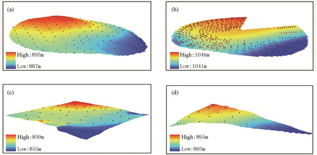
Figure 1. Soil sampling sites overlaid on the topography map for (a) Lamesa, (b) Halfway, (c) Ackerly I, and (d) Ackerly II. Soil samples from these sites were interpolated for use as the soil input for PALMS simulations.
Figure 2. This model provides a tool to effectively simulate the effects that different management practices have on the retention of rainfall and the resulting changes in soil water available for crop production.
Model Inputs. The PALMS model requires as input four layers of landscape information: soil texture, topography, crop type, and a surface mask (Figure 2). The model is executed with weather data on 15-minute time steps. All landscape data were created on 10 m grids as suggested by Bonilla et al. [22]. The model PALMS can accommodate up to 23 layers of soil information to a depth of 2.5 m at thicknesses from 0.02 m near the surface to 0.25 m at the bottom of the profile. At all sites, soil texture inputs were created from the soil core sampling. Point samples of soil texture for each depth were interpolated using the inverse distance weighted function; power four in ArcGIS (ESRI, Redlands, CA). Elevation points from GPS surveys were interpolated using the same procedure for soil texture data to create the required digital elevation model (DEM). The model PALMS includes corn and soybean crop models. In our case, and as a first approximation, soybean was used as a surrogate as the only C3 crop similar to cotton, and corn in similar fashion for C4 grain sorghum. Adjustments were made in plant populations and crop maturity types to simulate actual leaf area index and crop evapotranspiration (ETc).
Weather data were collected from the West Texas Mesonet (http://www.mesonet.ttu.edu) weather stations nearest to the field sites. For the Halfway location, the weather station was located at (34˚05'37.75" N, 102˚07' 04.46"W; 1,083 m elevation) 10 km south of Olton, TX, and 16 km southwest of the field site. Weather data for the Lamesa and Ackerly locations were collected from a weather station located at (32˚42'36.73"N, 101˚56'13.23"; 891 m elevation) 3 km southeast of Lamesa, TX. Measurements of air temperature and relative humidity, solar irradiance, rainfall, and wind speed were taken at a screen height of 2 m as described by Lascano [24]. Supplemental rainfall data were measured directly at the Ackerly and Lamesa sites with a tipping bucket rain gauge with an event data-logger (Model RG3, Onset Computer, Bourne, MA) and a similar rain gauge (Model TE525-L, Texas Electronics, Dallas, TX) attached to a data-logger (Model CR1000, Campbell Scientific, Logan, UT).
The PALMS management input file for each (Figure 2) simulation, which includes tillage, fertilizer, planting date and population, variety information, and initial soil conditions of water and temperature was created based on actual management practices or the best estimate of common practices if not all information was available. Information collected from soil data measurements taken at the weather stations previously mentioned was used to estimate initial values of soil water content and temperature profiles used as input.
Model Parameterization. Given the mechanistic nature of the PALMS model our calibration effort was to determine soil hydraulic parameters at each of the four locations (Figure 1) that optimized the agreement between measured and calculated values of soil water content. At each location we used two versions of the water solver routines. First, the original version as given by Molling et al. [10]; hereafter, referred to as “original” and second, using an adjusted soil water solver that accounted for dry, coarse textured soils characteristic to the SHP; hereafter, referred to as “updated.” These changes in the soil water
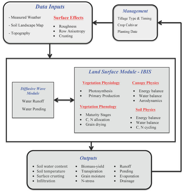
Figure 2. Flow diagram of the Precision Agricultural Landscape Modeling System (PALMS), adapted from Morgan et al. [19].
solver allowed for rapid infiltration of intense rainfall into dry, coarse textured soils similar to conditions that apply to the Amarillo soil series. The original version of PALMS allows soil water drainage in these scenarios because the forcing is in terms of diffusion and not potential. Specifically, changes to the soil water solver equation were made to alleviate the problem of soil water drainage when diffusion was in the opposite direction of water potential. The updated version reduces the diffusion term to a small number whenever diffusion was the opposite of potential. For the Halfway and Lamesa sites each original and updated version of PALMS was executed with five different soil hydraulic parameters: 1) Rawls pedotransfer functions, which are the default in PALMS [34]; 2) Rosetta pedotransfer function for the soil water retention curve (water potential vs. water content) [35]; 3) Rosetta pedotransfer function for the soil saturated hydraulic conductivity (Ks); 4) Rosetta pedotransfer function for Ks and soil water retention curve [35]; and 5) a corrected version of soil water retention curve and Ks. In addition, at the two Ackerly locations we used three measured soil hydraulic parameters, i.e., Ks, soil water retention, and Ks and soil water retention. In summary, two versions of the soil water solver (original and updated) were tested in combination with changes to soil hydraulic parameters (Table 1). Each version of the PALMS model, as shown in Table 1, represents different combinations of changes made to the soil water solver and the three soil hydraulic parameters at four locations. Additional details about the soil hydraulic properties used in our simulations at the Halfway and Lamesa locations are outlined in Tables 2 and 3. Measured and simulated soil hydraulic properties at both Ackerly locations are given by Alvarez-Acosta [36] and by Alvarez-Acosta et al. [37].
Specific water retention parameters used were θv at permanent wilting point (θpwp) and θv at field capacity (θfc). At all sites, soil water retention values were estimated using the Rosetta pedotransfer functions [35]. These functions are bundled as a computer program that uses neural network analysis to estimate water retention and Ks and unsaturated hydraulic conductivity, K(qv),
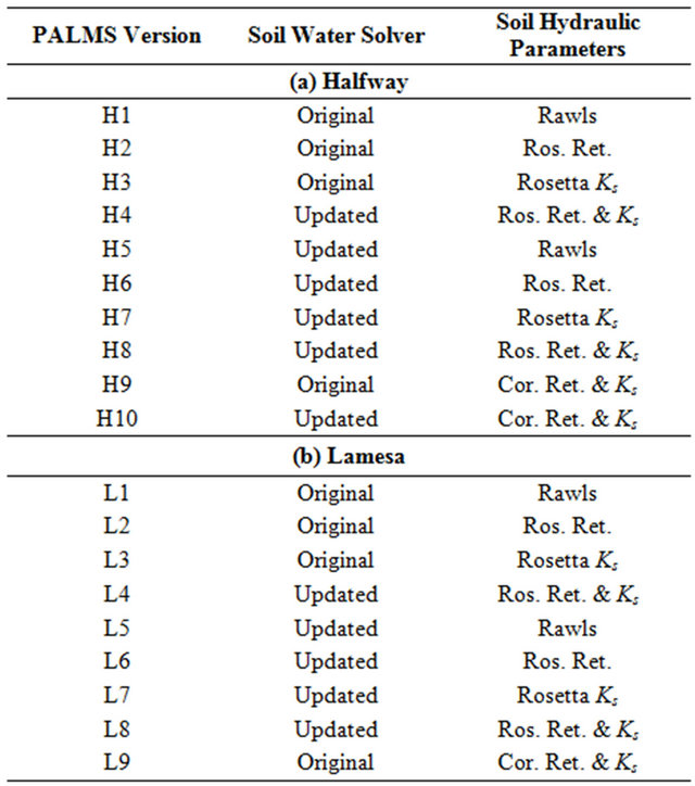
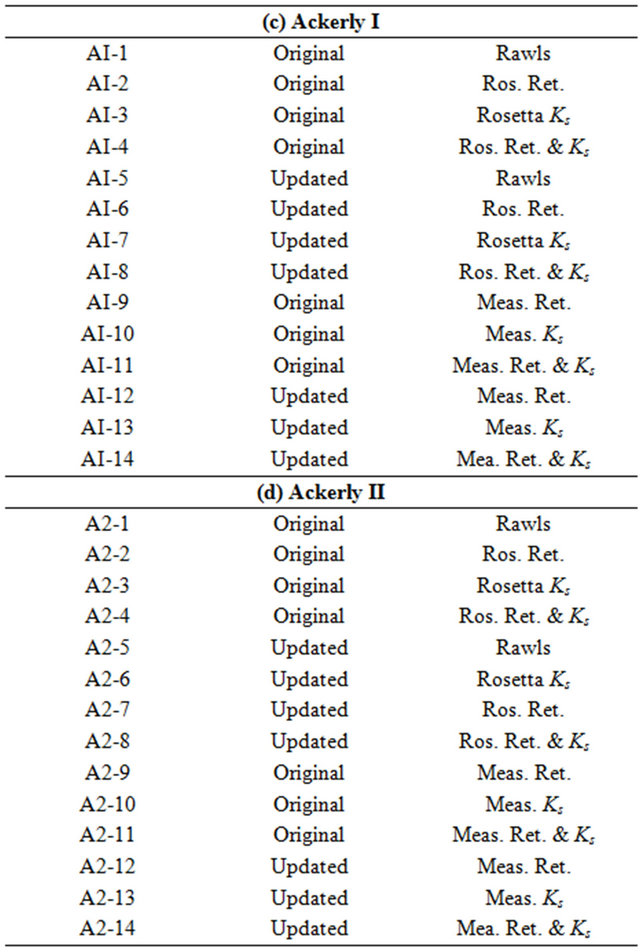
Table 1. The model PALMS versions tested at each experimental site: (a) Halfway, (b) Lamesa, (c) Ackerly I, and (d) Ackerly II.
using limited soil textural information. Specifically, Rosetta estimates residual soil water content (θr), saturated soil water content (θs), α (related to the inverse of the air entry suction), and n (a measure of the pore-size distribution) [37]. Estimates of θr and θs obtained with Rosetta [35] were converted to the appropriate calibration parameters for the model PALMS (θfc and θpwp) using a form of the Van Genuchten [37] relationship given by:
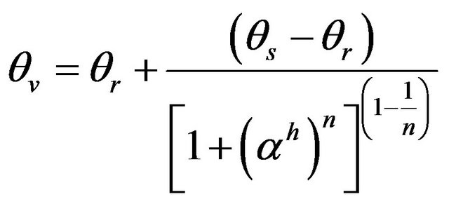 (1)
(1)
where h is pressure head (kPa), and α (1/kPa) and n are soil parameters described above. Changes in Ks and water retention parameters were made for each soil textural class at each experimental location, which represent three common soil series on the SHP. The Pullman series is represented at the Halfway location, while the Amarillo and Acuff series are most common at the Lamesa and Ackerly sites, respectively. For the Amarillo and Pullman soils, values for α and n were taken from Baumhardt et al. [28]. Soil water retention characteristics were measured from undisturbed cores of the Acuff soils [36,38] using methods described by Klute [39].
Different versions of the PALMS model were tested at the Halfway and Lamesa sites; respectively (Tables 1(a) and (b)) to determine which combination of soil water solver versions and soil hydraulic parameters resulted in the most accurate calculations of soil water content. For both Ackerly sites, the same set of parameter changes were made using Rosetta. Additionally, six more versions of PALMS were included using field measured hydraulic parameters from Acosta [38] (Tables 1(c) and (d)). The evaluation criteria for each PALMS version was to minimize the root mean squared difference (RMSD) between measured and calculated values of soil water content [26]. When all combinations of soil hydraulic parameters and soil water solver versions were tested, the model was deemed effective when RMSD values were ≤0.10 as suggested by Stockle et al. [40].
Evaluation of Calculated Values of Soil Water Content Obtained with PALMS. The PALMS model was executed for the 2000 and 2001 growing seasons at Lamesa and Halfway, respectively, and for the 2009-growing season at both Ackerly sites. Simulations were initialized 5 months before planting date to allow the model to equilibrate from the assigned initial input conditions of soil water and temperature. To assess the performance of PALMS under the specified environmental conditions, calculated values of θv were plotted against measured values at all sites. To evaluate the difference between measured and calculated values of soil θv we used the root mean square deviation (RMSD) [26,41] and is given by:
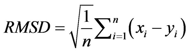 (2)
(2)
where xi is the calculated value of soil θv, yi is the corresponding measured value of soil θv, and n is the number of measurements. The RMSD represents the mean distance between simulation and measurement. Stockle et al. [40] suggested that RMSD values <0.10 indicate good agreement between measured and calculated values for a cropping system simulation model. Another statistical parameter used to evaluate calculated values obtained with PALMS is the mean square deviation (MSD), or the square of RMSD [26]. Furthermore, MSD is partitioned into the sum of three components, all calculated from regression coefficients. The first component is the squared bias (SB), which represents the bias of the simulation from the measurement given by:
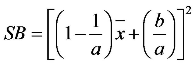 (3)
(3)
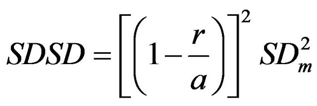
where a is the slope of the regression line, b is the y-intercept, and  is the mean value of xi. SB = 0 indicates measured and simulated values are identical. The second component is the squared difference between standard deviations (SDSD), which is the difference in the magnitude of fluctuation between the simulation and measurement, with a larger value of SDSD indicating a failure of the model to simulate the magnitude of fluctuation among the n measurements and is given by:
 (4)
(4)
where r is the correlation coefficient between the simulation and measurement, and SDm is the standard deviation of the measurement. The third and final component is the lack of positive correlation weighted by the standard deviations (LCS),
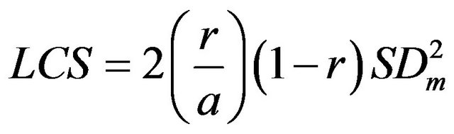 (5)
(5)
a large value of LCS indicates failure of the model to simulate the pattern of fluctuation across the n measurements. Note that in this analysis the mean squared deviation (MSD) is defined as [26]:
 (6)
(6)
3. Results and Discussion
3.1. Calculation of Soil Hydraulic Parameters Using Rosetta
All estimates of soil hydraulic properties used in PALMS were based solely on soil texture inputs as required by the Rawls [34] and Rosetta pedotransfer functions [35]. Soil hydraulic parameters were calculated in both Rawls and Rosetta using measurements of sand, silt and clay. However, from the results shown in Tables 2 and 3 it is clear that estimates obtained with the Rosetta pedotransfer functions based on soil texture information alone without any additional soil hydraulic parameters, demonstrate very little difference between Rosetta calculated parameters of different textural classes. This leads to the assumption that additional measured soil information (soil bulk density and soil water retention points) could cause Rosetta to produce more reliable output that would more accurately characterize the spatial and vertical variability of soil hydraulic characteristics at the simula-
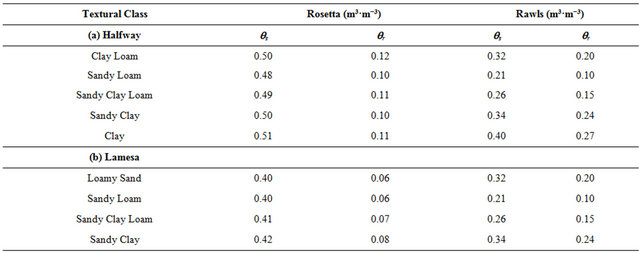
Table 2. Rosetta and Rawls simulated soil water retention values for textural classes found at the (a) Halfway site, and (b) Lamesa site. The θs and θr represent saturated and residual soil volumetric water content, respectively.
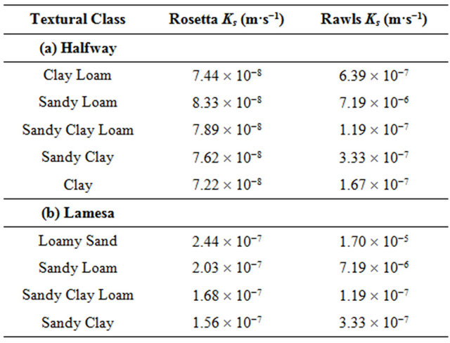
Table 3. Rosetta and Rawls simulated soil saturated hydraulic conductivity (Ks) for textural classes at (a) Halfway and (b) Lamesa sites.
tion sites. From this, additional Rosetta parameters were calculated using measured values of θr and θs from Baumhardt et al. [28] as additional input. The PALMS versions H9 and H10 for the Halfway location and L9 for the Lamesa location (Tables 1(a) and (b)) were created using these “corrected” soil hydraulic parameters under the assumption that more detailed input would improve Rosetta calculations. This follows the logic given by Schaap et al. [35] that Rosetta performance improves with the addition of more predictors (soil bulk density, soil water retention points) and is confirmed by the results of Alvarez-Acosta [38] and Alvarez-Acosta et al. [36].
3.2. Comparison of Calculated and Measured Soil Water Content
Halfway Location. As shown in Figure 3(a), average θv values ranged from 0.15 to 0.20 m3·m−3 throughout the growing season and are near the expected range of values for a Pullman soil as described by Baumhardt et al. [28]. Due to inaccuracies of θv measurements near the soil surface, inherent to neutron attenuation, we used measurements from the 0.15 to 0.45 m depth range. Since these measurements were taken below the surface horizon and as expected, they were not as responsive to irrigation and precipitation, and thus seasonal fluctuations in soil water were relatively small. As shown in Figure 3(a), the θv values calculated by PALMS did not show a consistent pattern when compared to measured values of soil θv, i.e., close at times and with large discrepancies at other times throughout the growing season. Several versions of the model matched the relative fluctuations of soil water, but absolute values were difficult to match. An updated version of PALMS with soil water solver corrections and Rawls (original) soil hydraulic parameters (H5) performed better than the original version. However, PALMS versions that excluded corrections to the soil water solver and included updated hydraulic parameters (H2 and H4) tended to produce smaller error throughout the season. This could be explained by the differences in soil hydraulic properties between the Pullman and Amarillo series. The Pullman series is hydraulically similar to the Midwest soils that have commonly been simulated with PALMS [10,19,22]. Additionally, model versions with updated soil water retention parameters (H9 and H10) generally performed better, as the lower wilting point for the clay loam textural class allowed the model to calculate lower values of soil water content typical in the 0.15 to 0.45 m depth range during the growing season. Further, PALMS was generally not sensitive to changes in Ks only. This could be explained by the fact that these soils rarely reach saturation, and in the SHP water movement is generally in the unsaturated state. Overall, the best-fit models (H2, H4, H9, and H10) calculated θv with RMSD values ranging from 0.05 to 0.08 m3·m−3 throughout the growing season (Figure 4(a)). The PALMS version H2 also demonstrated some ability to accurately represent the spatial distribution of θv at certain points in the growing season (data not shown). The consistency of the PALMS representation of the spatial distribution of soil water is naturally dependent on the model’s ability to calculate seasonal fluctuations in average soil water. As shown in Figure 5(a), the H4 version, which calculated soil water with the lowest seasonal RMSD, demonstrated a relatively large value of LCS at each sampling date, indicating a weakness in the model to accurately capture the pattern of the soil water fluctuation throughout the season. This was an expected result given the uncertainty on the values of soil hydraulic parameters used as input and on their spatial distribution. Fluctuating values of SDSD for the H4 version (Figure 5(a)) indicated that the model could accurately simulate large fluctuations in soil water, but was less reliable in characterizing smaller changes. Among the three error components, SDSD and LCS had the greatest effect on MSD. The very small portion of the MSD attributed to SB indicates that the RMSD values discussed earlier represent a high degree of accuracy obtained with the PALMS model. Although the seasonal RMSD of calculated soil water is acceptable, further work is needed to capture seasonal fluctuations in soil water for the Pullman soil series.
Lamesa Location. Because soil water was measured with a neutron probe at the same depth as was measured at the Halfway location, the seasonal fluctuations of θv at the Lamesa site were similar to that of the Halfway. Because soil water was measured below the surface hori-
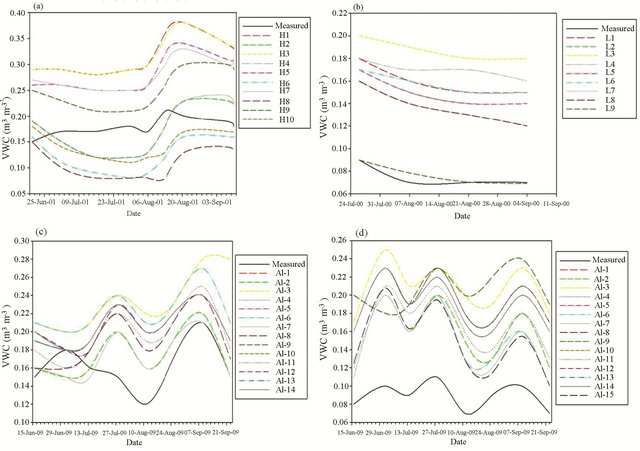
Figure 3. Measured vs. calculated soil volumetric water content (VWC, θv) throughout the growing seasons for the (a) Halfway site, (b) Lamesa site, (c) Ackerly I site, and (d) Ackerly II site.
zon, there was very little change in θv throughout the season (Figure 3(b)). This is most likely due to the fact that transpirational demand of a healthy crop during the growing season in the SHP will generally deplete most of the available soil water in the root zone, because the water needs of the crop normally exceed rain and irrigation. Figure 3(b) shows how all PALMS versions consistently overestimated θv. The simplest explanation for this discrepancy was that θv was too low (0.07 - 0.09 m3·m−3), and was out of range of most of the retention parameters calculated by the pedotransfer functions. Thus, an additional version (L9) was tested with θpwp values ranging from 0.01 to 0.03 m3·m−3. This version performed better (Figure 3(b)) than previous versions of PALMS, as the model calculated θv values in the range of measured values. As shown in Figure 4(b), all versions of the model other than L9 (PALMS version with adjusted values of θpwp) estimated soil water with 0.06 to 0.12 m3·m−3 error. L9 estimated absolute values of θv varied with a RMSD <0.02 (Figure 4(b)). In these conditions, all versions of the model generally matched the seasonal pattern of θv satisfactorily. This is demonstrated in Figure 5(b) by the small values of LCS for each soil water sampling date. The large values of SD in the middle of the growing season indicate some deviation between measured and simulated values, as demonstrated in Figure 3(b). Given the fact that the measured fluctuations of soil θv were as expected, given the texture of the soil and the sensitivity of the neutron probe, the model performed well. For the given soil type (Amarillo series) and environmental conditions, it would be useful to include measurements of θv nearer to the soil surface, as this range would respond to irrigation and precipitation and would include a wider range of soil water values. The PALMS version L9 also demonstrated some ability to accurately represent the spatial distribution of θv at certain points in the growing season (data not shown). The consistency of the PALMS representation of the spatial distribution of soil water is naturally dependent on the model’s ability to calculate seasonal fluctuations in average soil water. Because there is a small seasonal change in soil water at this location, PALMS was able to capture some of the spatial component of soil water distribution.
Ackerly I Location. Soil qv varied from ~0.15 to 0.20
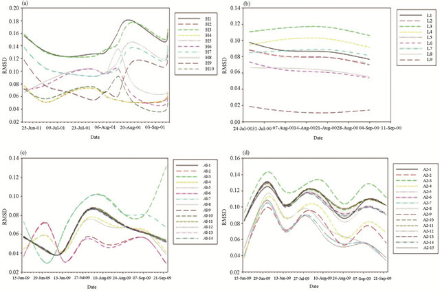
Figure 4. Seasonal fluctuations in RMSD for each version of PALMS tested at the (a) Halfway site, (b) Lamesa site, (c) Ackerly I site, and (d) Ackerly II site.
m3·m−3 throughout the growing season. In general, all PALMS versions matched the pattern of changes in θv after 1 August (Figure 3(c)). Error in soil water estimation was minimized the most with versions AI-2 and AI-6 (Figure 4(c)), both of which included changes in water retention parameters estimated by Rosetta. Similar to the Halfway and Lamesa locations, small values of LCS and SDSD indicated that the PALMS model (version AI-6) accurately calculated the pattern and magnitude of fluctuation throughout the growing season (Figure 5(c)). The large portion of the MSD attributed to SB indicated that the absolute values of soil water calculated by the model were inaccurate at times. However, the small values of LCS and SDSD mentioned above and apparent in Figure 3(c) suggested that the model could be very reliable if further changes were made to more accurately characterize absolute values of soil water. The model PALMS versions with measured Ks and soil water retention parameters behaved similarly regardless of the combination of parameters used. Although these versions reduced error early in the season, errors began to accumulate with fluctuations in θv. There was no response to changes in the soil water solver at this location. This soil
(Acuff) is similar to the Pullman series in that it is more generally a loam or sandy clay loam, rather than the fine sandy loam of the Amarillo series. This finer texture seems to generally respond more favorably to the original version of PALMS with no changes in the soil water solver.
Ackerly II Location. As shown in Figure 3(d), θv measurements varied considerably throughout the season, as expected. This simply illustrates the pattern obtained when θv is measured in the surface 0.15 m. All PALMS versions consistently overestimated θv at this location regardless of changes in retention parameters that reduced error at the Lamesa location (Figure 3(d)). Although seasonal values of RMSD were higher for all PALMS versions than at all other experimental locations (Figure 4(d)), PALMS was able to simulate the seasonal pattern of soil water fluctuation, as demonstrated by the small values of SDSD and LCS (Figure 5(d)). These results are very similar to those at the Ackerly I site, indicating that the PALMS simulated soil water will be very accurate in the Acuff soil series with further changes to better characterize absolute values of soil water.
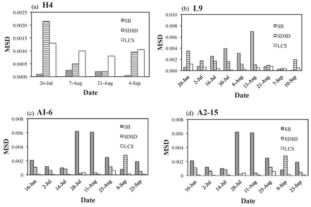
Figure 5. Mean Squared Deviation (MSD) components (simulation bias [SB], product of deviation of the means [SDSD], lack of positive correlation [LCS]) plotted for the best fit PALMS version for each experimental site: (a) PALMS version H4 (Halfway), (b) PALMS version L9 (Lamesa), (c) PALMS version AI-6 (Ackerly I), and (d) PALMS version A2-15 (Ackerly II).
4. Summary and Conclusions
Results from this study indicated that PALMS model calculated the seasonal water balance of the three major soil series (Pullman, Amarillo and Acuff) on SHP. In one particular case, (L9) PALMS accurately simulated absolute values of θv, while separately it was able to match the fluctuations in θv throughout a growing season, as shown at the Ackerly II location, where all other PALMS versions consistently overestimated θv. The magnitudes of fluctuations were accurately characterized as demonstrated by the small SDSD values shown in Figure 5, and shown visually in Figure 3(d). However, the model was unable to simulate θv fluctuations of >0.05 m3·m−3 without some error in the absolute values or time lag in soil water calculations, as demonstrated most notably at the Halfway and Ackerly I locations.
Semiarid regions, such as the SHP, are characterized by low precipitation and high evaporative demand, particularly during the growing season. These drought conditions are common and must be accounted for in crop simulations models. The discrepancy between measured and calculated values of soil water content obtained with PALMS indicates the importance of having the correct soil hydraulic properties that are used to calculate soil water movement in the profile. The PALMS model provides a framework that can be used as an irrigation management tool because the complexity of the interactions between soil, plant and environmental components are considered and integrated over time.
Relationships between management practices and crop yield are often variable between seasons and locations, depending on precipitation and other weather variables. Models such as PALMS are tools that have the potential to extend cropping systems field research ideas to other soils, crops, climates, and management practices. The PALMS model is a unique tool that combines mechanistic runoff and biosphere models with a crops module that addresses both crop production and the subsequent environmental consequences on agricultural landscapes. In water-limited regions such as the SHP, the ability to simulate crop growth in conjunction with runoff, infiltration, redistribution, etc. is necessary to fully understand how management practices will affect soil water at the production scale. More specifically, research related to irrigation management and tillage and crop rotation effects on soil water can be further developed without the concern of scaling up point models to the level of physical realism.
This research demonstrated that the simulation model PALMS can simulate soil water when soil properties are accurately characterized. It is then assumed that the model’s ability to calculate soil water content will allow researchers and growers to simulate runoff and erosion using processes within the model that have been previously evaluated. This ability to simulate the complex processes of the water balance at the landscape scale is of great importance to semiarid regions such as the SHP.
With future improvements in crop models and irrigation routines, the model PALMS will provide a valuable tool to evaluate both the short and long term effects of different soil, tillage, and irrigation management practices on soil and water conservation at the landscape scale in a region where water and its management are the most important factors to maintaining sustainable and profitable crop production.
5. Acknowledgements
This research was supported in part by the Ogallala Aquifer Program, a consortium between USDA-Agricultural Research Service, Kansas State University, Texas A & M AgriLife Research, Texas A & M AgriLife Extension Service, Texas Tech University, and West Texas A & M University.
REFERENCES
- H. P. Mapp, “Irrigated Agriculture on the High Plains: An Uncertain Future,” Western Journal of Agricultural Economics, Vol. 13, No. 2, 1988, pp. 339-347.
- R. L. Baumhardt and R. J. Lascano, “Rain Infiltration as Affected by Wheat Residue Amount and Distribution in Ridged Tillage,” Soil Science Society of America Journal, Vol. 60, No. 6, 1996, pp. 1908-1913. doi:10.2136/sssaj1996.03615995006000060041x
- D. Bosch, T. Potter, C. Truman, C. Bednarz and T. Strickland, “Surface Runoff and Lateral Subsurface Flow as a Response to Conservation Tillage and Soil-Water Conditions,” Transactions of the American Society of Agricultural Engineers, Vol. 48, No. 6, 2005, pp. 2137-2144.
- L. D. Norton and L. C. Brown, “Time-Effect on Water Erosion for Ridge Tillage,” Transactions of the American Society of Agricultural Engineers, Vol. 35, No. 2, 1992, pp. 473-478.
- P. W. Unger and J. J. Parker, “Evaporation Reduction from Soil with Wheat, Sorghum, and Cotton Residues,” Soil Science Society of America Journal, Vol. 40, No. 6, 1976, pp. 938-942. doi:10.2136/sssaj1976.03615995004000060035x
- C. Rodgers, J. Mecikalski, C. Molling, J. Norman, C. Kucharik and C. Morgan, “Spatially Distributed Hydrologic-Biophysical Modeling: Applications in Precision Agriculture,” 24th Conference on Agricultural and Forest Meteorology, Davis, 14-18 August 2000, pp. 86-87.
- J. Zhu, C. L. S. Morgan, J. M. Norman, W. Yue and B. Lowery, “Combined Mapping of Soil Properties Using a Multi-Scale Tree-Structured Spatial Model,” Geoderma, Vol. 118, No. 3-4, 2004, pp. 321-334. doi:10.1016/S0016-7061(03)00217-9
- R. D. Connolly, “Modelling Effects of Soil Structure on the Water Balance of Soil-Crop Systems: A Review,” Soil & Tillage Research, Vol. 48, No. 1, 1998, pp. 1-19. doi:10.1016/S0167-1987(98)00128-7
- B. Diekkrüger, D. Söndgerath, K. C. Kersebaum and C. W. McVoy, “Validity of Agroecosystem Models: A Comparison of Results of Different Models Applied to the Same Data Set,” Ecological Modeling, Vol. 81, No. 1-3, 1995, pp. 3-29. doi:10.1016/0304-3800(94)00157-D
- C. C. Molling, J. C. Strikwerda, J. M. Norman, C. A. Rodgers, R. Wayne, C. L. S. Morgan, G. R. Diak and J. R. Mecikalski, “Distributed Runoff Formulation Designed for a Precision Agricultural Landscape Modeling System,” Journal of the American Water Resources Association, Vol. 41, No. 6, 2005, pp. 1289-1313. doi:10.1111/j.1752-1688.2005.tb03801.x
- C. A. Jones and J. R. Kiniry, “CERES-Maize: A Simulation Model of Maize Growth and Development,” Texas A & M University Press, College Station, 1986.
- W. D. Batchelor, J. O. Paz and K. R. Thorp, “Development and Evaluation of a Decision Support System for Precision Agriculture,” Proceedings of the 7th International Conference on Precision Agriculture and Other Precision Resources Management, Minneapolis, 25-28 July, 2004, pp. 2005-2009.
- K. C. DeJonge, A. L. Kaleita and K. R. Thorp, “Simulating the Effects of Spatially Variable Irrigation on Corn Yields, Costs, and Revenue in Iowa,” Agricultural Water Management, Vol. 92, No. 1-2, 2007, pp. 99-109. doi:10.1016/j.agwat.2007.05.008
- D. K. Borah and M. Bera, “Watershed-Scale Hydrologic and Nonpoint-Source Pollution Models: Review of Mathematical Bases,” Transactions of the American Society of Agricultural Engineers, Vol. 46, No. 6, 2003, pp. 1553- 1566.
- R. E. Smith and J. Y. Parlange, “A Parameter-Efficient Hydrologic Infiltration Model,” Water Resources Research, Vol. 14, No. 3, 1978, pp. 533-538. doi:10.1029/WR014i003p00533
- I. Takken, G. Govers, V. Jetten, J. Nachtergaele, A. Steegen and J. Poesen, “Effects of Tillage on Runoff and Erosion Patterns,” Soil & Tillage Research, Vol. 61, No. 1, 2001, pp. 55-60. doi:10.1016/S0167-1987(01)00178-7
- J. France and J. H. M. Thornley, “Mathematical Models in Agriculture,” Butterworth & Co, London, 1984.
- C. Müller, “Modelling Soil-Biosphere Interactions,” CABI Publishing, New York, 2000.
- C. L. S. Morgan, J. M. Norman, C. C. Moiling, K. McSweeney and B. Lowery, “Evaluating Soil Data from Several Sources Using a Landscape Model,” In: Y. A. Pachepsky, et al., Eds., Scaling Methods in Soil Physics, CRC Press, New York, 2003, pp. 243-260.
- J. Bouma, “Using Soil Survey Data for Quantitative Land Evaluation,” Advances in Soil Science, Vol. 9, 1989, pp. 177-213. doi:10.1007/978-1-4612-3532-3_4
- A. B. McBratney, B. Minasny, S. R. Cattle and R. W. Vervoort, “From Pedotransfer Functions to Soil Inference Systems,” Geoderma, Vol. 109, No. 1, 2002, pp. 41-73. doi:10.1016/S0016-7061(02)00139-8
- C. A. Bonilla, J. M. Norman and C. C. Molling, “Water Erosion Estimation in Topographically Complex Landscapes: Model Description and First Verifications,” Soil Science Society of America Journal, Vol. 71, No. 5, 2007, pp. 1524-1537. doi:10.2136/sssaj2006.0302
- C. A. Bonilla, J. M. Norman, C. C. Molling, K .G. Karthikeyan and P. S. Miller, “Testing a Grid-Based Soil Erosion Model Across Topographically Complex Landscapes,” Soil Science Society of America Journal, Vol. 72, No. 6, 2008, pp. 1745-1755. doi:10.2136/sssaj2007.0310
- R. J. Lascano, “A General System to Measure and Calculate Daily Crop Water Use,” Agronomy Journal, Vol. 92, No. 5, 2000, pp. 821-832. doi:10.2134/agronj2000.925821x
- R. J. Lascano, C. H. M. van Bavel and S. R. Evett, “A Field Test of Recursive Calculation of Crop Evapotranspiration,” Transactions of the American Society of Agricultural and Biological Engineers, Vol. 53, No. 4, 2010, pp. 1117-1126.
- K. Kobayashi and M. U. Salam, “Comparing Simulated and Measured Values Using Mean Squared Deviation and its Components,” Agronomy Journal, Vol. 92, No. 2, 2000, pp. 345-352. doi:10.2134/agronj2000.922345x
- G. W. Gee and J. W. Bauder, “Particle-Size Analysis,” In: A. Klute, Ed., Methods of Soil Analysis, 2nd Edition, American Society of Agronomy and Soil Science Society of America, Madison, 1986, pp. 383-411.
- R. L. Baumhardt, R. J. Lascano and D. R. Krieg, “Physical and Hydraulic Properties of a Pullman and Amarillo Soil on the Texas South Plains,” Texas Agricultural Experiment Station, Lubbock, 1995.
- C. Hignett and S. R. Evett, “Neutron Thermalization,” In: J. H. Dane and G. C. Topp, Eds., Methods of Soil Analysis, Soil Science Society of America, Madison, 2002, pp. 501-521.
- S. R. Evett and J. L. Steiner, “Precision of Neutron Scattering and Capacitance Type Soil Water Content Gauges from Field Calibration,” Soil Science Society of America Journal, Vol. 59, No. 4, 1995, pp. 961-968. doi:10.2136/sssaj1995.03615995005900040001x
- H. Li, R. J. Lascano, J. Booker, L. T. Wilson and K. F. Bronson, “Cotton Lint Yield Variability in a Heterogeneous Soil at a Landscape Level,” Soil & Tillage Research, Vol. 58, No. 3-4, 2001, pp. 245-258. doi:10.1016/S0167-1987(00)00172-0
- R. G. Blake and K. H. Hartge, “Bulk Density,” In: A. Klute, Ed., Methods of Soil Analysis, American Society of Agronomy and Soil Science Society of America, Madison, 1986, pp. 363-382.
- J. A. Foley, I. C. Prentice, N. Ramankutty, S. Levis, D. Pollard, S. Sitch and A. Haxeltine, “An Integrated Biosphere Model of Land Surface Processes, Terrestrial Carbon Balance, and Vegetation Dynamics,” Global Biogeochemical Cycles, Vol. 10, No. 4, 1996, pp. 603-628. doi:10.1029/96GB02692
- W. Rawls, L. Ahuja and D. Brakensiek, “Estimating Soil Hydraulic Properties from Soils Data,” In: M. Th. Van Genuchten, Ed., Indirect Methods for Estimating Hydraulic Properties of Unsaturated Soils, University of California, Riverside, 1992, pp. 329-341.
- M. G. Schaap, F. J. Leij and M. Th. van Genuchten, “ROSETTA: A Computer Program for Estimating Soil Hydraulic Parameters with Hierarchical Pedotransfer Functions,” Journal of Hydrology, Vol. 251, No. 3-4, 2001, pp. 163-176. doi:10.1016/S0022-1694(01)00466-8
- C. Alvarez-Acosta, R. J. Lascano and L. Stroosnijder, “Test of the Rosetta Pedotransfer Function for Saturated Hydraulic Conductivity,” Open Journal of Soil Science, Vol. 2, No. 3, 2011, pp. 203-212. doi:10.4236/ojss.2012.23025
- M. Th. Van Genuchten, “A Closed-Form Equation for Predicting the Hydraulic Conductivity of Unsaturated Soils,” Soil Science Society of America Journal, Vol. 44, No. 5, 1980, pp. 892-898. doi:10.2136/sssaj1980.03615995004400050002x
- C. Alvarez-Acosta, “Use of Precision Agricultural Landscape Modeling (PALMS) for Estimating the Effects of Cultural Practices on Infiltration, Runoff and Erosion,” M.Sc. Thesis, Wageningen University, Wageningen, 2009.
- A. Klute, “Water Retention: Laboratory Methods,” In: A. Klute, Ed., Methods of Soil Analysis, American Society of Agronomy and Soil Science Society of America, Madison, 1986, pp. 635-686.
- C. O. Stockle, S. A. Martin and G. S. Campbell, “Cropsyst, a Cropping Systems Simulation Model: Water-Nitrogen Budgets and Crop Yield,” Agricultural Systems, Vol. 46, No. 3, 1994, pp. 335-359. doi:10.1016/0308-521X(94)90006-2
- R. L. Ott and M. Longnecker, “Introduction to Statistical Methods and Data Analysis,” 5th Edition, Duxbury Press, Pacific Grove, 2001.
NOTES
*The US Department of Agriculture (USDA) prohibits discrimination in all its programs and activities on the basis of race, color, national origin, age, disability, and where applicable, sex, marital status, familial status, parental status, religion, sexual orientation, genetic information, political beliefs, reprisal, or because all or part of an individual’s income is derived from any public assistance program.
1Mention of this or other proprietary products is for the convenience of the readers only and does not constitute endorsement or preferential treatment of these products by USDA-ARS.