Open Journal of Modern Hydrology
Vol. 2 No. 4 (2012) , Article ID: 23417 , 8 pages DOI:10.4236/ojmh.2012.24009
Assessing Stream Health in the Chesapeake Basin Using the SHARP Model
![]()
1Department of Meteorology, Pennsylvania State University, University Park, USA; 2NOAA/NWS/MDL, Silver Spring, Maryland, USA; 3Ocean and You, Oakland, USA; 4Spatial Information Technologies, Inc., State College, USA.
Email: tnc@meteo.psu.edu, amy.haase@noaa.gov, cynthia.cudaback@gmail.com, m_anderson14@hotmail.com
Received July 14th, 2012; revised August 30th, 2012; accepted September 12th, 2012
Keywords: Stream Health; Water Quality; Chesapeake Bay Basin; Nutrient; Sediment Loads
ABSTRACT
An assessment of stream health within the Chesapeake Bay Basin can be made using the Stream Health and Runoff Potential (SHARP) model, which is based solely on the relationship between land cover and stream constituents: Total phosphorus (TP), total nitrogen (TN), and total suspended sediment (TSS). While not intended to compete with more complex models that utilize a range of specific input data, SHARP’s advantage is that it requires little input, is easily applied, and can show whether a stream or watershed is likely to be impacted (impaired). The model allows the user to define a watershed boundary on screen within which a stream health index (SHI), concentrations of TP, TN and TSS, percentages of five land cover types, a color-coded land cover snapshot, impervious surface area and fractional vegetation cover are output. The paper describes SHARP, its output and an overview of how it can be used.
1. Introduction
The Stream Health and Runoff Potential (SHARP) model was designed to show where and to what degree watersheds are liable to be impaired by high concentrations of total nitrogen (TN), total phosphorus (TP) and total suspended sediment (TSS) within the Chesapeake Bay Basin. The model’s basis is statistical, relating land cover percentages to concentrations of these three constituents. SHARP is not meant to compete with more comprehensive watershed models such as the SPARROW model [1] or the GWLF model [2,3] see also the web site: http://www.avgwlf.psu.edu/overview.htm.
Rather, the model allows the user to quickly assess the health of a selected watershed or stream basin with a minimum of input. Both the SPARROW and GWLF models are more physically based than SHARP and require a variety of environmental data as input. GWLF can be accessed on line; SHARP is also executed on line. Output contains estimates of TN, TP, and sediment loads for the designated area, a stream health index, area percentages of urban, woodland, water, short vegetation and bare soil/scrub, plus impervious surface area and fractional vegetation cover. It provides a color coded snapshot of the area based on a Landsat image classification for the year 2000. SHARP also includes a separate runoff potential component, a separately downloaded module executable on one’s desk computer; the runoff component will not be discussed in this paper. Instead, we address only the development of the stream health module, including its statistical validation, and describe briefly the method for extracting the information and interpreting the output.
2. Data Analysis
An important finding was made by Sheeder and Evans [4]. They compiled historical stream flow and waterquality data to create annually-averaged nitrogen, phosphorus and sediment loads for various watersheds in Pennsylvania. Daily flow rates were obtained from the US. Geological Survey for a ten year period between 1989 and 1999 [5] and nutrient concentrations were collected by the Pennsylvania Department of Environmental Protection (PaDEP). Historical water-quality data were compiled for either the 1987 to 1994 or the 1990 to 1996 time interval depending on data availability. In-stream nutrient concentrations were paired with corresponding flow rates for 42 Pennsylvania watersheds (Figure 1). Simple mass balance relationships were used to calculate yearly averaged nutrient and sediment loads [5].
These loads were averaged over the 10-year sampling period and used as response variables to generate statistical regression equations between land-use/land cover
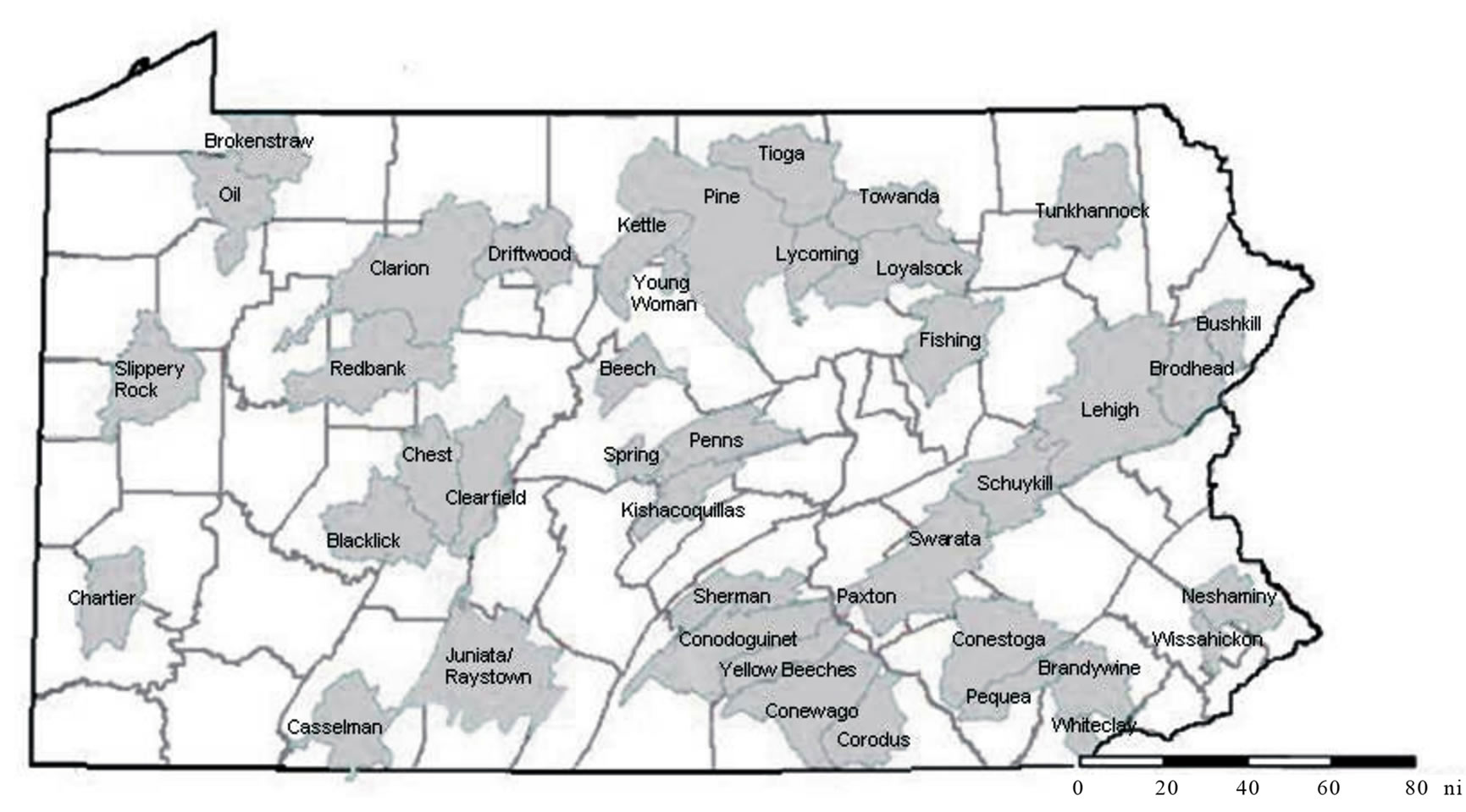
Figure 1. Forty-two Pennsylvania watersheds in grey with county boundaries underlying.
percentages and nutrient and sediment loads. Not all watersheds have all three measured water quality parameters; a total of 16 watersheds in Pennsylvania contained all three constituents.
Concentrations of nitrogen, phosphorus and sediment loads are of great interest to regulatory agencies for making assessments of stream health. For this reason, [4] determined values for stream impairment, using biological assessments conducted by the PaDEP. Their assessment covered 17 unimpaired and 12 impaired watersheds, distinguished by the health of the aquatic ecosystem. They discovered that impairment responded to rather sharply delineated thresholds of the three constituents, above which the stream was found to be impaired. They chose the midpoint between the median impaired and unimpaired loads as a threshold value for each constituent. The threshold loads are: nitrogen, 8.64 kg/HA; phosphorus, 0.30 kg/HA and sediment 785.29 kg/HA [4]. In our study, these threshold values were used to create a simple way for watershed managers to interpret nutrient and sediment loads in terms of overall health of a stream.
These same constituent data were related to land cover analyses based on classifications done on Landsat imagery.
Several prior studies have provided remotely-sensed data used in our project. Statewide percentage of Impervious Surface Area (ISA) and land-cover maps for the Commonwealth of Pennsylvania using Landsat data with 30 m resolution for the year 2000 available on the Pennsylvania Spatial Data Analysis (PASDA) web site [6].
Image classification was performed by Dr. Eric Warner of Penn State Institutes of the Environment (PSIE), from which we determined fractional vegetation cover from the raw Normalized Difference Vegetation Index (NDVI) data and ISA using the methodology described by [7]. These data for Pennsylvania consist of percentages of urban, wooded, short vegetation, bare soil/scrub vegetation, and water, plus the ISA and fractional vegetation cover for pixels at 30 m resolution. Additional land cover and ISA analyses were provided by Dr. Stephen Prince [8] at the University of Maryland for the entire Chesapeake Bay Watershed outside of Pennsylvania constituent data. Using Pearson’s relations, he found that developed land, which is linearly related to ISA, was correlated with nitrogen (R = 0.394) and phosphorus (R = 0.879). Wooded land was anti-correlated with nitrogen (R = −0.768), and agricultural land was positively correlated with nitrogen (R = 0.697).
Chang [9] measured correlations between land use and water quality for 38 Pennsylvania watersheds using the same stream data provided by Evans [5]. Similarly, phosphorus was anti-correlated with woodland (R = −0.420) and very weakly correlated with agricultural land (R = 0.094). Other strong predictors of nitrogen concentration were the elevation and slope of the watershed, as well as runoff and temperature suggesting that cold, swift mountain streams have superior water quality [9].
3. Input Data
ISA and fractional percentage of wooded and ISA were determined from the year 2000 Landsat imagery for each watershed shown in Figure 1. Agricultural land (vegetation) was not used as a predictor for the following reason: vegetation, woodland and urban (i.e., percent ISA) comprise almost the entire image, so that any two of these three land cover variables effectively prescribe the area coverage for the third. Adding a third category of vegetation does not increase the accuracy of the regression equations if percent woodland and %ISA are also prescribed.
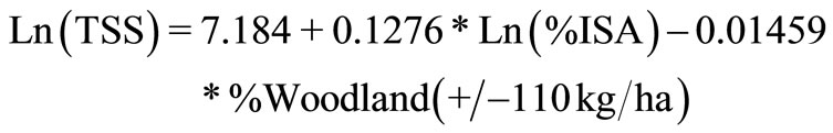
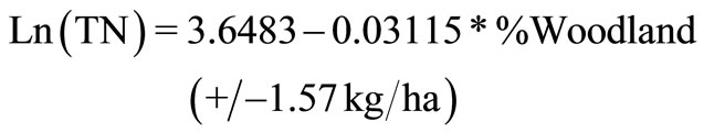
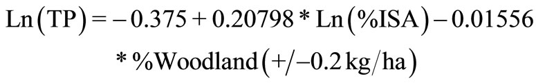
These data were related statistically to the measured stream constituents. An analysis was made relating measured constituent data, TN, TP and TSS, to ISA and percent woodland. The best relationships were those which exhibited the highest correlations (R-squared), the lowest P-scores, and a reasonable degree of statistical normality [10]. The correlations between predictors (%ISA and %woodland) and response variables (measured TP, TN and TSS) were calculated to determine which variables should be used in the empirical model. All concentrations appear to be exponentially related to woodland coverage, with significantly lower concentrations of the measured constituents in wooded areas. The strongest correlations having the lowest P-scores among variables were: ln(TN), to %woodland, ln(TP) to ln (%ISA) and %woodland, and ln(TSS) to ln(%ISA) and %woodland. Multiple predictor R-squared values for these relationships, specifically between each of the constituents and the land use variables, were all about 0.65. Relationships apply, of course, only within the range of measurements: the woodland fractions between 20% and 100%, and ISA fractions between 0 and 10%; a few small watersheds contained greater than 15% ISA. Measured TSS loads were a few hundred to a few thousand kilograms per hectare per year (kg/ha/yr). TN loads were between 0.5 kg/ha/yr and 40 g/ha/yr, and TP loads ranged from a 0.1 kg/ha/yr to 3.2 kg/ha/yr. Thus, either one or two predictors were selected for relating land use/land cover to loadings of TP, TN and TSS, %ISA and %woodland for the 42 watersheds (Figure 1). Having determined the best possible empirical relationships between the
 (1)
(1)
 (2)
(2)
 (3)
(3)
measured percentages of ISA and woodland cover for Pennsylvania, the results were extended to apply to the entire measured nutrient and sediment loads and the measured percentages of ISA and woodland cover for Pennsylvania, the results were extended to apply to the entire Chesapeake Bay Basin. The degree to which this extrapolation is valid is discussed in the validation section of this paper. Optimum relationships are described by the regression Equations (1)-(3), where the numbers in parentheses refer to the standard deviations in the original measured data for the 42 watersheds.
4. Statistical Regression Equations
Figure 2 shows %woodland and %ISA, where the curves illustrate the threshold concentrations of nutrient or sediment from [4]. Of the three variables, phosphorus has
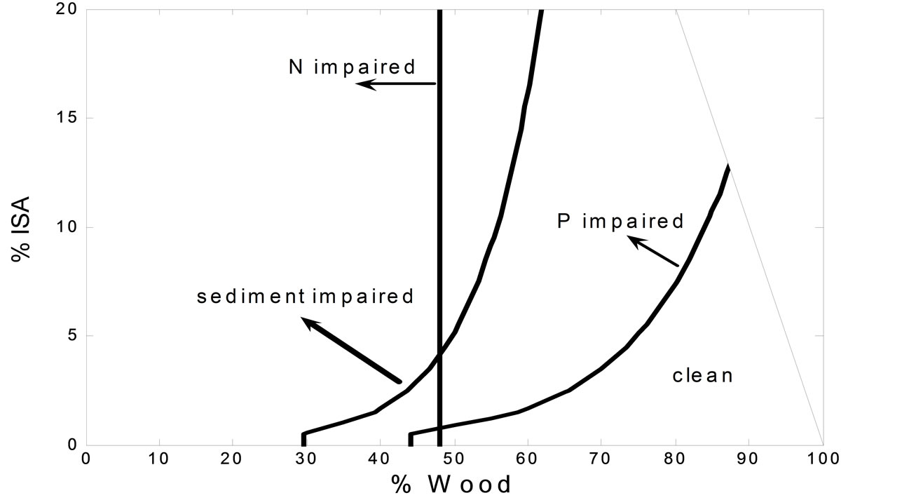
Figure 2. Statistical regression equations plotted in parameter space illustrating the thresholds between impaired and unimpaired watersheds for the three constituents, here referred to as N (nitrogen), P (phosphorus) and sediment.
the smallest un-impacted region, indicating that phosphorus concentrations are most sensitive to urbanization, especially at low values of %woodland. The vertical line for N (TN) signifies its lack of sensitivity to %ISA, whereas P (TP) is sensitive to both %ISA and %woodland. The sensitivity to both environmental parameters is underscored by Sheeder and Evans [4], who found that impaired watersheds had median land use fractions of 11% urban (analogous to ISA) and 40.5% forest (located entirely in the impaired domain of Figure 2), while median unimpaired watersheds were 1.4% urban and 78.0% forest (located entirely within the unimpaired domain of the figure). The figure suggests that N is insensitive to urbanization, unlike P whose loading seems to depend in part on runoff from urban surfaces. Note, however, that the threshold results imply some ambiguity in which any of the three constituents might appear on different sides of the impaired-unimpaired thresholds. We have found, however, that this situation does not arise very often and, when it does, all three constituents are close to their respective thresholds.
5. Stream Health Index (SHI)
In order to provide an easily interpretable number describing whether and to what degree a watershed or stream is impaired, we have developed a simple Stream Health Index (SHI) based on the threshold values for constituent loads developed by Sheeder and Evans [4] and the statistical results referred to by Equations (1)-(3). SHI quantifies the degree of stream impairment without subjecting the reader to graphs showing enormous scatter of points without an understanding of what the values signify. The SHI value assigned to each constituent (TN, TP and TSS) ranges from –2 to +2. A positive score indicates an unimpaired stream, a negative score an impaired stream. Each pollutant is given a score based on the magnitude greater than or less than the threshold value. Total range for the three constituents combined is from plus to minus 6.
The narrow range for neutral (SHI = 0) reflects the very sharp thresholds found by Sheeder and Evans [2004]. For loads between 10% below (above) threshold and half (double) the threshold value receives a score of plus (minus) one for clean (impaired), while loads greater than (less than) double (half) the thresholds receive a score of minus (plus) two. Values are added for each of the three constituents to create a scale from –6 to +6 for the SHI, the former pertaining to a highly impaired watershed and the latter a pristine watershed. These relationships are shown in Table 1" target="_self"> Table 1.
6. Validation
Constituent data published for the SPARROW model for TN and TP [1] and measurement data based on [11] and [5] were used to compare with SHARP and to generally evaluate the SHI generated from Equations (1)-(3) for the TN and TP concentrations. Close agreement between SPARROW, the reference model, and SHARP would suggest a high degree of confidence in the latter.
SPARROW requires a great deal of information about individual watersheds, including land use, temperature, terrain slope, stream density, wetland, irrigated land, precipitation, irrigation water use, fertilizer application rates, livestock production and atmospheric deposition. It predicts nutrient concentrations with some accuracy, explaining almost 90% of the data variability; it does not predict sediment concentrations.
In evaluating the SHARP model using measurements and comparing it to SPARROW we were interested to know if the regression equations cited above have validity within the Chesapeake Bay Basin both inside and outside of Pennsylvania. To do this we included SPARROW output and measurements of TN and TP, those published by the USGS [11] and by [12]. In comparing nutrient loads from two different models with each other and with measurements, it was necessary to reconcile watershed results on three different scales. The SPARROW model watersheds were, in general, smaller than the HUC-11 watersheds used for SHARP. By combining SPARROW model outputs from small, adjacent watersheds, we were able to replicate the size and location, and thereby the fractions of land-use for 35 of the 42 Pennsylvania watersheds used in SHARP. Similar compositing of watershed boundaries was required in order to reconcile the USGS data with both SHARP and SPARROW for areas within the Chesapeake Bay Basin outside of Pennsylvania.
Because of the enormous scatter of the raw measurements including many outliers, we believe that the best way to make model comparisons is to use SHI indices in contingency tables [10] based only on either the TN and TP constituents combined or on individual constituents
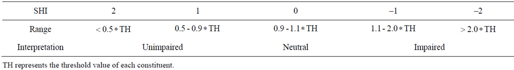
Table 1. Stream heath index relationships.
common to both SHARP and SPARROW in 2005. As such and without TSS, the range of SHI is only from –4 to +4. Thus, values of SHI being compared can differ by as much as 8 units (e.g., –4 versus +4). Perfect agreement (e.g., –4 versus –4) would lie along the axis of the matix (the shaded boxes), shown for 35 watersheds in Pennsylvania in the example given in Figure 3. Here, 12 of the values show perfect agreement, while 27 lie within one index value for a comparison between SHARP and SPARROW output. Thus, 77% of the points fall within plus or minus one index value for the SHI.
Table 2 summarizes the overall comparisons between models and measurements based only on the two constituents, TN and TP. Referring to the example given in Figure 3, perfect agreement within the comparison is defined as occurring along the diagonal. Good agreement is defined as occurring within one box from the one-toone diagonal. The greater the frequencies along or near this diagonal, the greater the agreement between models and/or observations.
Table 2 shows SHI values broken down in into individual (TN or TP) constituents, as well as the two combined. Note that SHARP somewhat out performs SPARROW inside Pennsylvania when compared with measurements, with the former having a score of 88 percent versus 69 percent agreement for SPARROW. As in the example above, SHARP has a 77% agreement with SPARROW. Outside Pennsylvania SHARP performs
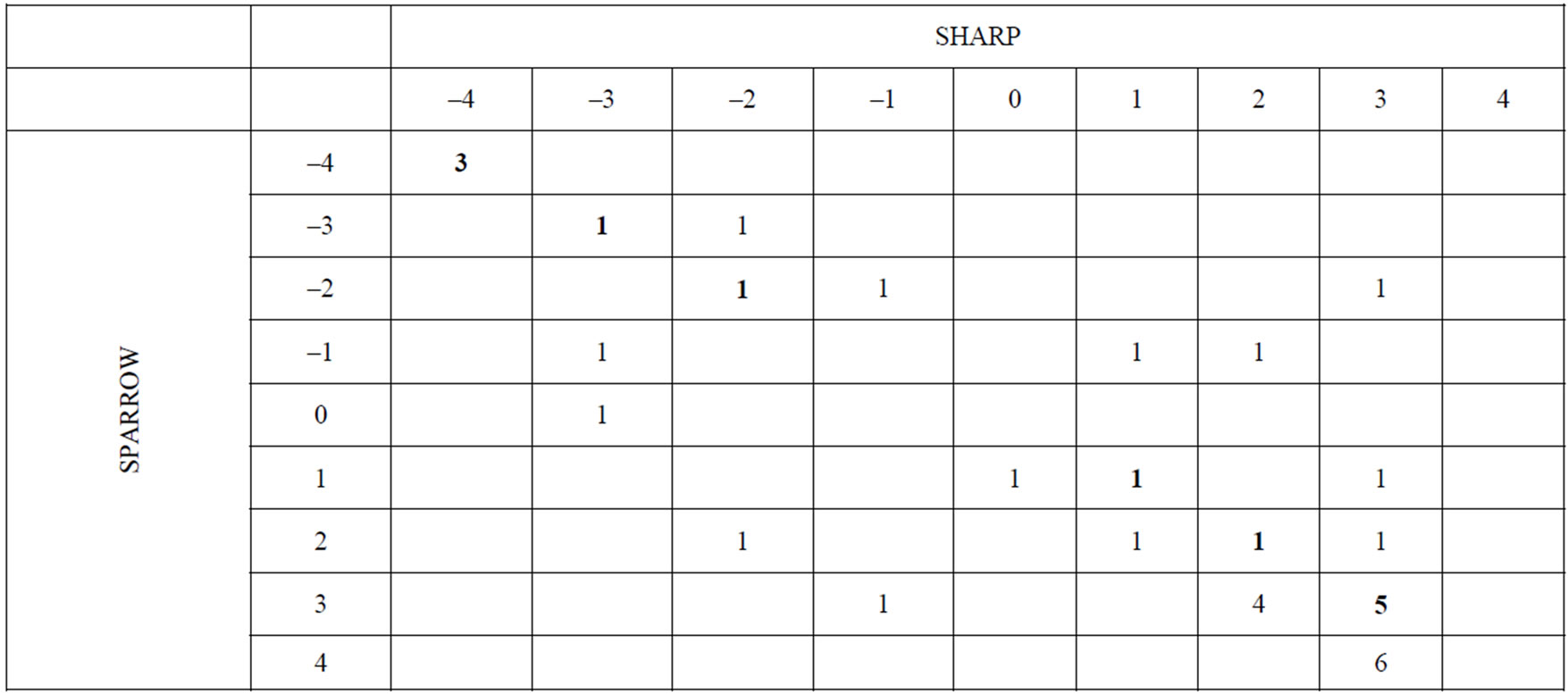
Figure 3. Contingency table for individual or combined TN and TP; a comparison for SPARROW versus SHARP.
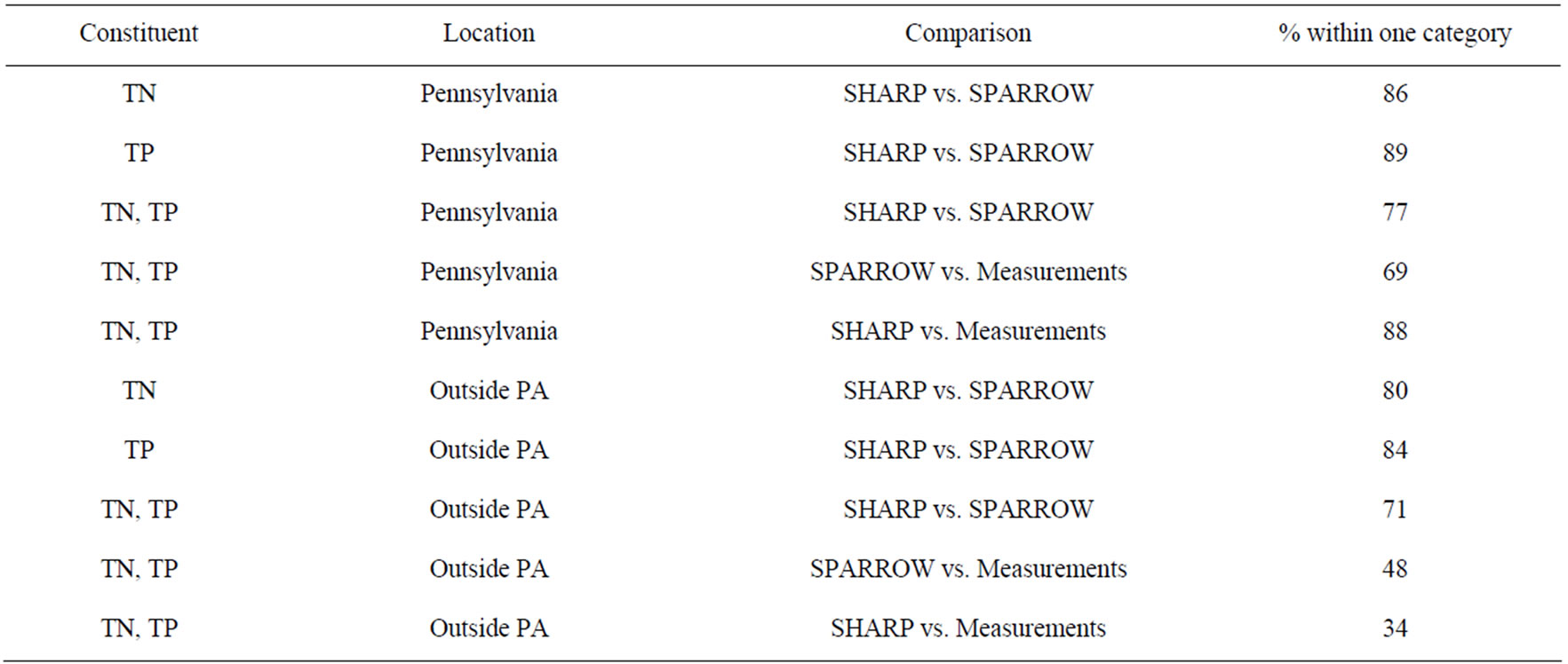
Table 2. Comparisons of SHI between models (Equations (1)-(3)) and measurements of constituents TN and TP, individually or combined.
somewhat poorer than SPARROW (48 versus 34 percent), although both models do worse than in Pennsylvania. Agreement between the two outside Pennsylvania is 71%. Why this degradation outside Pennsylvania occurred for both models is not clear. As both SHARP and SPARROW seem to suffer almost equally from the same degradation, we believe that the reduction in agreement between model and measurement may be due to factors other than the models themselves, such as a poorer quality measurements or our method of forcing watershed sizes to be equal for both measurement and model.
One additional evaluation of SHARP was done. In 2005 approximately 50 watershed experts were invited to Penn State in order to learn how to use the SHARP model. Each expert was instructed to select his or her own watershed and perform an analysis in which SHI (and other parameters) could be assessed. All participants who responded agreed that the SHI constituted a realistic assessment of their particular watershed’s health.
7. Execution of SHARP on Line
The SHARP web site can be accessed at: http://www.sharp.psu.edu/analysis.htm which contains a description of SHARP, its documentation, and two web pages that allow the user to run the model either in Pennsylvania or the greater Chesapeake Bay. These two sites differ only on the geographic extent they cover not the functionality they provide.
The user can zoom in to the watershed of interest and manually draw the watershed using a USGS topographic map with contour lines as a base map, or the user can define the watershed outlet and let the USGS’s Pennsylvania StreamStats application delineate the watershed draining to the outlet (http://water.usgs.gov/osw/streamstats/pennsylvania.html) in Pennsylvania [12] and [13]. On the Chesapeake Bay page, the user must manually delineate the watershed as there is no StreamStats application that covers the entire Bay.
SHARP is simple to operate and requires no data input or technical knowledge, other than being able to locate a stream of interest on a USGS topographic map. Figure 4" target="_self"> Figure 4 illustrates two screens displayed in retrieving the results from the Pennsylvania SHARP page for a particular stream basin, that of Slab Cabin Run in Centre County, PA. The first screen image (top figure) shows the initial map displayed on the Pennsylvania page at the address cited. The map then allows the user to zoom in on the desired location. Once zoomed in to the approximate location, the USGS topographic map can be turned on by selecting it in the blue box at the top right of the map.
If a manual delineation is desired, the Delineate Water shed menu at the top left of the page is used. The first step is to select Draw Watershed from the menu and then draw the watershed boundary on the map using the contour lines. Each point along the boundary is created by clicking once on the map. The boundary is completed by double clicking on the map. If the boundary needs to be edited, the Edit Watershed the watershed menu item can be selected. Then the boundary can be clicked on the begin editing. After edited is completed, the Stop Editing menu item should be selected. When the boundary is correct, the Retrieve Loading Estimates menu is selected, opening a form to create the SHARP loading estimates. A final step using a button on the output table is required to compute additional results, such as the SHI; an optional command brings up the color-coded land use/land cover image of the watershed. If a StreamStats delineation is desired, the Delineate Outlet menu at the top left of the page is used. In order to get accurate results from the StreamStats application, the outlet must be placed where StreamStats defines the stream to be (head of arrow on right hand side of Figure 4). This is not always where the topo map shows the stream to be. To make sure the outlet is located correctly, turn on the Streams (NHD) layer in the blue box at the upper right of the map. These are the stream locations as defined by the USGS 1:24,000 National Hydrography Dataset (NHD). The Define Outlet menu is used to place the outlet on an NHD stream segment. If the outlet location is incorrect, the Edit Outlet menu item is used to move it to the correct location. When the outlet location is correct, the Retrieve Watershed menu item is used to retrieve the outlet from the Pennsylvania StreamStats application. When the watershed is retrieved it loads automatically on the map. The final step is to select the Retrieve Loading Estimates menu item, as in the example above, to open a form to create the SHARP loading estimates.
The Chesapeake Bay page works the same way, except the initial map covers the entire bay, and there is no option to create an outlet and use StreamStats to delineate the watershed.
8. Summary
SHARP appears to yield a realistic assessment of watershed impairment. Although SHARP is not meant to supplant any of these more complex nutrient models currently under development or in use, it can serve as a very useful tool, allowing the user quick and easy way to make at least a preliminary assessment of the biological viability and land cover distribution for any of the tens of thousands streams and watersheds within Pennsylvania and the Chesapeake Bay Basin.
Execution of SHARP on line is relatively simple, re quiring no technical expertise or an extensive data base.
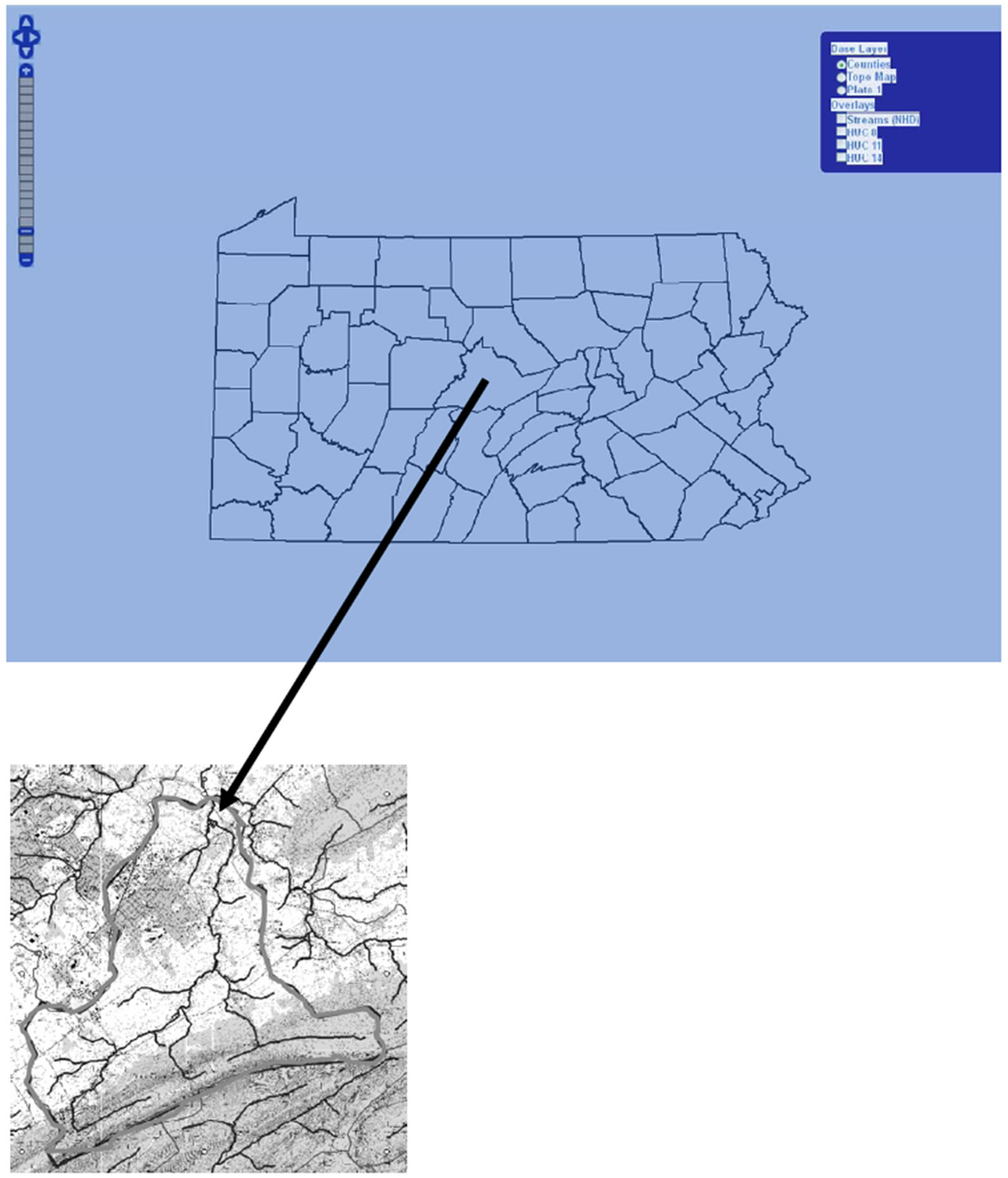
Figure 4. Two steps in delineating a watershed. Pennsylvania with counties (top figure) and an extracted watershed (highlighted) with streams (lower figure); see text for details. Arrow points from its location to the neck of watershed.
Watershed boundaries are defined in SHARP on screen, either by clicking on a stream outlet or by tracing a closed boundary. SHARP is unique in that it provides a wider range of output products for the watershed in question than just nutrients, such %ISA, %woodland and other products extracted from the Landsat image. These output products are:
1) Estimates of nutrient (TN, TP) and sediment concentrations;
2) Impervious surface cover and fractional vegetation cover;
3) A stream health index (SHI), allowing the user to quickly assess the biological viability of the watershed/ stream;
4) Land cover percentages for five basic types as classified from the Landsat image for the year 2000: (urban, woodland, short vegetation (agriculture), bare soil, water);
5) A snapshot satellite image of the area color coded to show the five land cover types;
6) A separate, downloadable runoff module is not a subject for this paper.
SHARP is also accompanied by a users guide to assist in executing the model.
9. Acknowledgements
Many people helped us create SHARP. Financial assistance was provided by the Pennsylvania Department of Environmental Protection (PaDEP), the CARA group, the Chesapeake Bay Foundation, the NASA Space Grant program, Jack Watson with the Penn State Cooperative Extension and Outreach Program, the USGS, the University of Maryland, (such as professor Prince) and the Growing Greener program, which provided seed money. A recent upgrade to SHARP was made possible by an additional grant from PaDEP.
REFERENCES
- S. D. Preston, R. A. Smith, G. E. Schwartz, R. R. Alexander and J. W. Brakebill, “Spatially Referenced Regression Modeling of Nutrient Loading in the Chesapeake Bay Watershed,” Proceedings of the First Federal Interagency Hydrologic Modeling Conference, Las Vagas, 19-23 April 1998, Vol. 1, pp. 143-150.
- D. A. Haith and L. L. Shoemaker, “Generalized Watershed Loading Functions for Stream Flow Nutrients,” Water Resources Bulletin, Vol. 23, No. 3, 1987, pp. 471-478.
- B. M. Evans, D. W. Lehning, K. J. Corradini, G. W. Petersen, E. Nizeyimana, J. M. Hamlett, P. D. Robillard and R. L. Day, “A Comprehensive GIS-Based Modeling Approach for Predicting Nutrient Loads in Watersheds,” Journal of Spatial Hydrology, Vol. 2, No. 2, 2002, pp. 1-18. www.spatialhydrology.com
- S. A. Sheeder and B. M. Evans, “Estimating Nutrient and Sediment Threshold Criteria for Biological Impairment in Pennsylvania Watersheds,” JAWRA Journal of the American Water Resources Association, Vol. 40, No. 4, 2004, pp. 881-888. doi:10.1111/j.1752-1688.2004.tb01052.x
- B. M. Evans, “Private Communication,” 2002.
- Pennsylvania State University Spatial Data Access (PASDA), 2005. http://www.pasda.psu.edu
- T. N. Carlson and D. A. J Ripley, “On the Relationship between NDVI, Fractional Vegetation Cover, and Leaf Area Index,” Remote Sensing of Environment, Vol. 62, No. 3, 1997, pp. 241-252. doi:10.1016/S0034-4257(97)00104-1
- S. Prince, “Private Communication,” 2005.
- H. Chang, “Spatial Variations of Nutrient Concentrations in Pennsylvania Watersheds,” Journal of the Korean Geographical Society, Vol. 27, 2002, pp. 535-550.
- H. A. Panofsky and G. W. Brier, “Some Applications of Statistics to Meteorology,” Mineral Industries Extension Services, University Park, Pennsylvania, 1958.
- USGS Report, “Yields and Trends of the Nutrients and Total Suspended Solids in Non-Tidal Areas of the Chesapeake Bay Basin, 1985-1995,” Water Resources Investigation Report 98-4192, US Geological Survey, US Department of the Interior, 1998.
- J. W. Brakebill, S. D. Preston and S. Martucci, “Digital Data Used to Relate Nutrient Inputs to Water Quality in the Chesapeake Bay Watershed, Version 2.0,” 2001. http://md.water.usgs.gov/publications/ofr-01-251/sparrow.htm
- M. A. Roland and M. H. Stuckey, “Regression Equations for Estimating Flood Flows at Selected Recurrence Intervals for Ungaged Streams in Pennsylvania,” US Geological Survey Scientific Investigations Report 2008- 5102, 2008, 57 p.