Open Journal of Modern Hydrology
Vol. 2 No. 3 (2012) , Article ID: 21225 , 10 pages DOI:10.4236/ojmh.2012.23007
Climate Change Impacts on the Extreme Rainfall for Selected Sites in North Western England
![]()
School of the Built Environment, Liverpool John Moores University, Liverpool, UK.
Email: M.E.Abdellatif@2010.ljmu.ac.uk
Received March 9th, 2012; revised April 28th, 2012; accepted May 24th, 2012
Keywords: Artificial Neural Network; Climate Change; Downscaling; Extremes Frequency Analysis Generalised Linear Model; Generalised Pareto Distribution
ABSTRACT
Impact and adaptation assessments of climate change often require more detailed information of future extreme rainfall events at higher resolution in space and/or time, which is usually, projected using the Global Climate Model (GCM) for different emissions of greenhouse concentration. In this paper, future rainfall in the North West region of England has been generated from the outputs of the HadCM3 Global Climate Model through downscaling , employing a hybrid Generalised Linear Model (GLM) together with an Artificial Neural Network (ANN). Using two emission scenarios (A1FI and B1), the hybrid downscaling model was proven to have the capability to successfully simulate future rainfall. A combined peaks-over-threshold (POT)-Generalised Pareto Distribution approach was then used to model the extreme rainfall and then assess changes to seasonal trends over the region at a daily scale until the end of the 21st century. In general, extreme rainfall is predicted to be more frequent in winter seasons for both high (A1FI) and low (B1) scenarios, however for summer seasons, the region is predicted to experience some increase in extreme rainfall under the high scenario and a drop under the low scenario. The variation in intensity of extreme rainfall was found to be based on location, season, future period, return period as well as the emission scenario used.
1. Introduction
Extreme events have greater impacts on the lives of communities and hence investigation of extreme events is crucial for impact assessment and adaptation studies. These studies require data of fine temporal-spatial resolutions to capture wide ranges of climate regime.
Most existing systems of water management and other infrastructure have been designed under the assumption that climate is stationary. This basic concept on which engineers work, assumes that climate is variable, but with properties of this variability being constant with time and occur around an unchanging mean state. This assumption of stationary conditions is still common practice for design criteria for (the safety of) new infrastructure, even though the notion that climate change may alter the mean, variability and extremes of relevant weather variables is now widely accepted [1]. It is possible to account for non-stationary conditions (climate change) in extreme value analysis, but scientists are still debating the best way to do this. Nevertheless, adaptation strategies to climate change should now begin to account for the decadal scale changes (or low-frequency variability) in extremes observed in the past decades, as well as projections of future changes in extremes such as those which are obtained from climate models.
Confidence has increased that some extremes will become more frequent, more widespread, and/or more intense during the 21st century [2]. As a result, the demand for information services on weather and climate extremes is growing. The sustainability of economic development and living conditions depends on our ability to manage the risks associated with extreme events. Therefore, there is a need for climate change scenarios to obtain data for impact and vulnerability assessment, for awareness development, for decision making in setting polices and for adaptation strategies [3]. For many studies, information derived directly from global climate model outputs may not be of sufficient spatial or temporal resolution to represent changes within a specific region, hence downscaling is required.
A recent study in the UK, which employed climateprediction.net (CPDN) model simulations from the BBC Climate Change Experiment for the A1B emission scenario [4], was conducted to shed light on the behaviour of future climate. It was found that the time of detectable change depends on the season, with most model runs indicating that a change to winter extremes in precipitation may be detectable by 2080, and that a change to summer extreme precipitation will not be detectable by 2080 [4]. Another study in the UK by Osborn et al. [5] who used gamma distribution to fit daily precipitation amount, reported that extreme precipitations have increased in frequency in winter and decreased during summer. Although these findings are consistent with those from UK Climate Prediction 2009 (UKCP09) study (for the same emission scenario) in winter, however for summer, the changes are less clear. The central estimate (50th percentile) suggests that the summer extremes may become slightly more frequent in the future for most locations, but there is a large level of uncertainty. The 10th percenttile change for summer suggests that the rainfall events will become much less frequent [6].
This paper is an extension for the above studies in order to develop quantifiable insights on the impacts of global climate change on extremes daily rainfall at appropriate scales during the winter and summer for SRES scenarios A1FI (high emission of greenhouse gases) and B1 (low emission). It is focused on North West of England and uses data from two urban catchments.
2. Data Used
Daily rainfall data from two stations in the region of North-western England was used for the purposes of this study. The first is Tower Wood station in Windermere Catchment (in the upper part of the region) and the second is Worleston station in the Crewe Catchment (in the lower part of the region) (see Figure 1). The two catchments represent relatively two different climates, with Windermere in the North having more annual rainfall
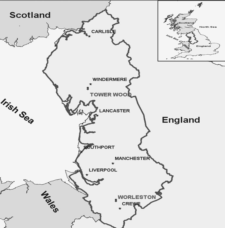
Figure1. Rainfall gauges used in the case study.
data sets are obtained from the Environment Agency for England and Wales for the period 1961-2001.The largescale observed climatic predictors data set is derived from the National Centre for Environment Predictions (NCEP/NCAR) for the same period of 1961-2001. Climate variables corresponding to the future climate change scenarios, which are on the same resolution as the NCEP predictors, are extracted from the Hadley Centre 3rd generation (HadCM3) Global Climate Model for future period 2010-2099.The selection of the future time slices up to 2080s allows assessment of the climate change impact on rainfall extremes in near and distant future.
3. Future Rainfall Prediction
In this paper the statistical downscaling methodology adopted, broadly follows a two stage approach to model daily rainfall. The first stage is related to the rainfall occurrence and the second stage is related to the amount of rainfall associated with a wet day. For the first stage, the methodology employs a regression based method of the generalised linear model (GLM) to represent rainfall occurrence and an artificial neural network (ANN) for the second stage. As is the case with all statistical downscaling methods, the hybrid GLM-ANN methodology used here assumes that the derived relationships between the observed predictors (climate variables) and predictand (i.e. rainfall) will remain constant under conditions of climate change and that the relationships are time-invariant [7,8].
The hybrid GLM-ANN downscaling methodology is started by first screening for predictors for the rainfall from all climate variables obtained from NCEP data at grid point level. The predictors are selected from a range of candidate predictors based on significance and strength of their correlation coefficients with the rainfall. Stepwise regression is applied during the selection process as it yields the most powerful and parsimonious model as has been shown by previous studies [9,10]. In order to remove any inconsistencies associated with the presence of small rainfall values, a threshold of 0.3 mm is applied to the data as rainfall values less than this threshold are considered to be dry days and represented with 0. Those equal to or greater than the threshold are considered wet days and represented with 1 to form a series of binary values for the rainfall occurrence model which has been screened with the predictors. All predictor variables are normalised to account for any biases that may occur in the modelled data.
The logistic regression is one of a large class of GLM [11] which is often used to model the probability of rainfall occurrence as a function of predictors (atmospheric variables) in statistical downscaling applications. In the present study, the logistic regression has been employed to model wet and dry sequences of rainfall at each station. The description of logistic regression explained below is given by [12].
If Pi denotes the probability of rain for the ith case in the data set, conditional on the covariate vector  (climate variables); then the model is given by,
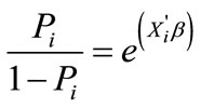 (1)
(1)
wheree = base of the natural logarithms
β = coefficients estimated from the data As a general result of the properties of the exponential family distribution, the maximum likelihood estimator of GLM parameters can be found robustly using the Newton-Raphson algorithm [13].
To test the performance of the occurrence model, the Percent Correct (PC) and Heidke Skill Score (HSS) indices proposed by [14] are used as a check for the Bias (B). These indices can be obtained from a 2 × 2 contingency table as shown in Table 1 [14,15] as below:
1) Number of events which are forecasted and actually occurred (a)
2) Number of events which are forecasted but not occurred (b)
3) Number of events which are not forecasted but occurred (c)
4) Number of events which are not forecasted and not occurred (d)
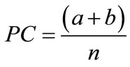 (2)
(2)
PC ranges from zero (0) for no correct forecasts to one (1) when all forecasts are correct.
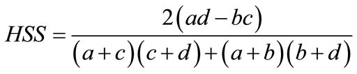 (3)
(3)
HSS = 1 for a perfect forecast; HSS = 0 shows no skill or poor model. If HSS < 0, the forecast is worse.
 (4)
(4)
If B = 1 (means forecast is unbiased), if B >1 (there is an over forecast), and if B < 1 (there is an under forecast). where a, b, c, and d are as defined in Table 1.
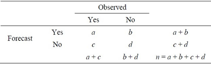
Table 1. Contingency table for possible outcomes of the occurrence model.
For the amount model, a multi-layer feed forward artificial neural network (MLF-ANN) model was used to build a non-linear relationship between the observed rainfall amount series and the same selected set of climatic variables (predictors) used for the rainfall occurrence model.
The rainfall series used to calibrate this model was re-sampled with the derived occurrence model, some of which may return zero amounts despite the fact that the original series of rainfall indicates a wet day.
Levenberg-Marquardt [16] optimization algorithm was used to train the network. The algorithm was designed to speed up the training process which would take longer if the usual back-propagation algorithm was used. In this study MATLAB 7.11 software has been used to model the two processes.
The developed hybrid GLM-ANN seasonal rainfall downscaling models were then used to simulate seasonal future rainfall using a set of input variables generated by global circulation models (for A1FI and B1 scenarios for emissions) as predictors (this set corresponds to the NCEP predictors used in building the downscaling model). The occurrence model was then used with inputs from the HadCM3 predictors to identify wet and dry days of the future rainfall based on the occurrence model. If the probability resulting from the occurrence model is equal to or greater than a specific threshold (specified during building of the occurrence model) then the amount estimated by the GLM-ANN model is taken as the rainfall amount for that particular day and if the probability of the occurrence is less than this threshold, the rainfall amount is taken as zero or a dry day. Prediction of future rainfall was produced for three future periods of the 2020s, 2050s and 2080s.
To avoid bias that may occur from use of GCM variables to simulate future rainfall, the so called Scaling (or direct approch) Method [17] is used to correct the future rainfall values. The scaling method can be expressed in mathematical terms as:
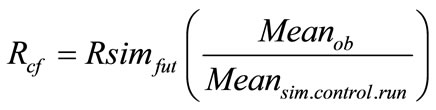 (5)
(5)
whereMeanob is mean observed rainfall for 1961-1990, and Meansim.control.run is mean simulated rainfal of the GCM for the control period.
4. Modelling Extremes Rainfall
Rainfall frequency analysis is performed for current and future climate by fitting the peaks-over-threshold (POT) model, which represents the behavior of exceedances above a high threshold and the threshold crossing process. Under suitable conditions, and using a high enough threshold, extremes identified in this way resulted in a generalized Pareto (GP) distribution. This was introduced by [18] and has applications in a number of fields including reliability studies and analysis of environmental extreme events.
The cumulative distributions function, F(x), of the GPD, where k ≠ 0 is given as
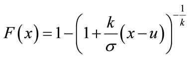 (6)
(6)
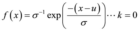
For k = 0 the GPD is just an exponential distribution:
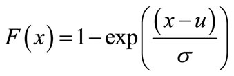 (7)
(7)
where, x is the random variable, x > u, and u = a threshold, k = shape parameter, σ = scale parameter and probability density function, f(x), for GPD is given as,
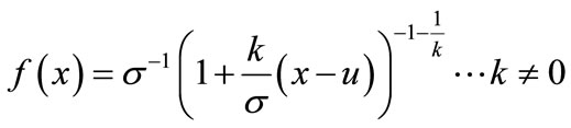 (8)
(8)
 (9)
(9)
4.1. Threshold Selection
The fundamental problem when fitting GPD is selection of an appropriate threshold for the peak-over-threshold calculation. Parameters of the GPD are very sensitive to the threshold selection and must be set high enough that only true peaks, with Poisson arrival rates, are selected. If this is not the case, the distribution of selected extremes will fail to converge to GPD asymptote. On the other hand, the threshold must be set low enough to ensure that enough data are selected for satisfactory determination of distribution parameters [19].
Most methods developed to solve the threshold problem are difficult to implement, therefore efficient methods to find the appropriate threshold is needed [20]. There are two distinct ways for refining the selected threshold that have been applied in this study. These two ways are initiated by fixing a threshold, a priori and abstracting from the data every peak value exceeding that threshold and then refining it. The refining methods are:
1) Parameter stability plots: These are plots of shape and scale parameters of the GPD obtained for a range of thresholds and then investigated for the stability of their estimates. The appropriate threshold value can be chosen by selecting the lowest value at which the graph becomes constant [21,22].
2) Mean Residual plot: This is a plot of the mean excess over threshold as a function of threshold. For a GPD model, the graph should plot as a straight line taking into account the 95% confidence bounds, and the appropriate threshold value can be chosen by selecting the suitable value above which the graph is straight line [23,24].
4.2. Fitting GPD
The GPD parameters are estimated by the maximum Likelihood Estimation (MLE) method, as it is known that if the sample size is large (which is the case in this study) the MLE is preferred because of its efficiency [25,26]. The estimation of parameter is applied using the extremes toolkit [27]. The following is the log likelihood equation, LL(x, σ, k), used in fitting the GPD for k ≠ 0:
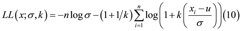 (10)
(10)
The Extreme Quantile (XT) estimation for a specified Return Period T is given by:
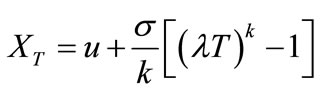 (11)
(11)
4.3 Model Diagnostics for GPD Fitting
It is necessary to check goodness of fit of a statistical distribution to extreme values series. The goodness of fit and reliability of GPD to simulate future extreme values are tested in this study using the following four diagnostics [27]:
1) Probability plot: Equation (6 or 7) is used to calculate the fitted value of the theoretical cumulative distribution function (cdf), which is plotted against the empirical value of the cdf for each data point. The values in the sample of data should be arranged in ascending order. In the case of perfect fit the plot is approximately linear.
2) Quantile plot: The empirical quantile of the sample data is arranged in ascending order and is plotted against the fitted quantile. Equation (6 or 7) is used for estim ating this fitted quantile from its inverse. The plot should be linear if the model is well representative by the data.
3) Return level plot: Equation (11) is used for estimating the return level which is plotted against the return period. Confidence intervals can be added to the plot to increase its informativeness. If the GPD is suitable for the data; the empirical estimate of return level should be within the confidence interval in a reasonable way.
4) Density plot: This is a comparison of the probability density function (pdf) of the fitted model with the histogram of extreme rainfall data. Equation (8 or 9) for estimating the fitted (pdf) is superimposed on the histogram, and matching between the two plots, is checked visually.
5. Results and Discussion
5.1. Downscaling Model Performance
Table 2 shows set of predictors which have been selected based on strength of their correlation with rainfall, for the two seasons in each of the two stations.
Definition of each of the predictor that appears in Table 2 is given in Table 3. It can be observed from the data in Table 2 that the lag forward and exponential transformations were used in some predictors because they produced better corelation with the observed rainfall. The most dominant predictors for the rainfall in the two stations, for both seasons, are relative humidity (rhum), vorticity (p_z) at surfaces, 500 hp and 850 hp levels, and surface meridional velocity (p_v). The vorticity (p_z at different levels) tends to be the most important predictor (judged by its strong correlation with rainfall in all stations). This is consistant with findings of studies carried out in this region by [10,28]. Zonal velocity (p-u) at 850hp, mean sea level (msl) and surface air flow strength (p_f) are ranked second in terms of dominance for both seasons. Near surface specific humidity (shum) and surface divergence (p_zh) appear to be dominant at Worleston in winter and Tower Wood in summer, respectively. Generally, 8 predictors have been found more suitable in predicting rainfall occurance and amount at the two stations, as dictated by the correlation coefficient of the stepwise regression model.
Table 4 shows the performance of the seasonal occurrence models for each station in terms of the Heidke Skill Score (HSS) and Percent Correct (PC) indices, as well as their Bias (B). The models have been calibrated and validated using daily rainfall data for a 27 year (1961-1987) period and a 14-year (1988-2001) period, respectively. The indices values shown in Table 4 suggest that both of the Tower Wood seasonal models are more accurate than the Worleston ones.This is attributed to the nature of rainfall in the Lakes District (where the Windermere catchment falls) as rainfall is more frequent with high intensity. The results in Table 4 also confirm that all developed occurrence models are capable of predicting rainfall occurrence with sufficient accuracy as dictated by higher values of PC (>70%) for both calibration and verification periods.
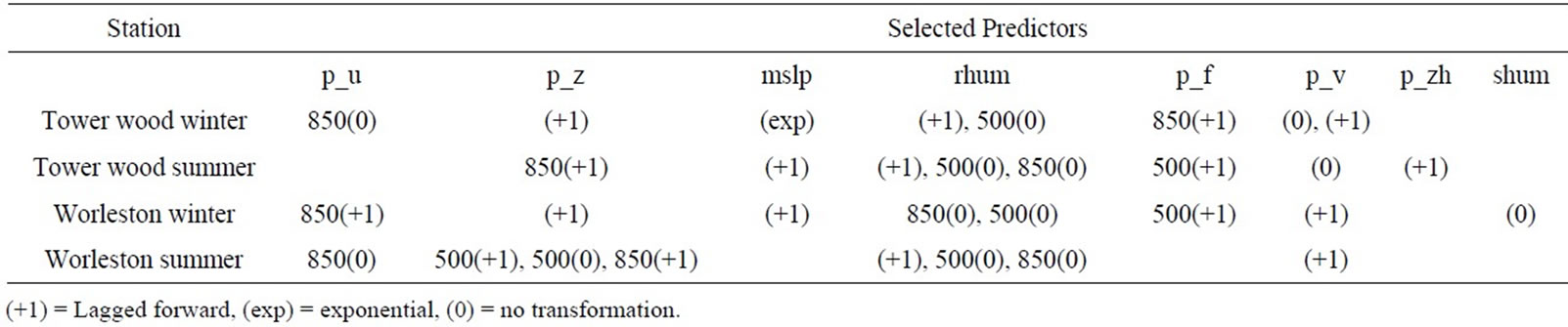
Table 2. Selected large-scale climate variables for winter & summer seasons at each station.
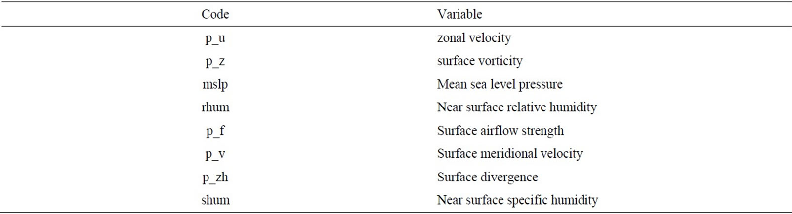
Table 3. Predictors definition.
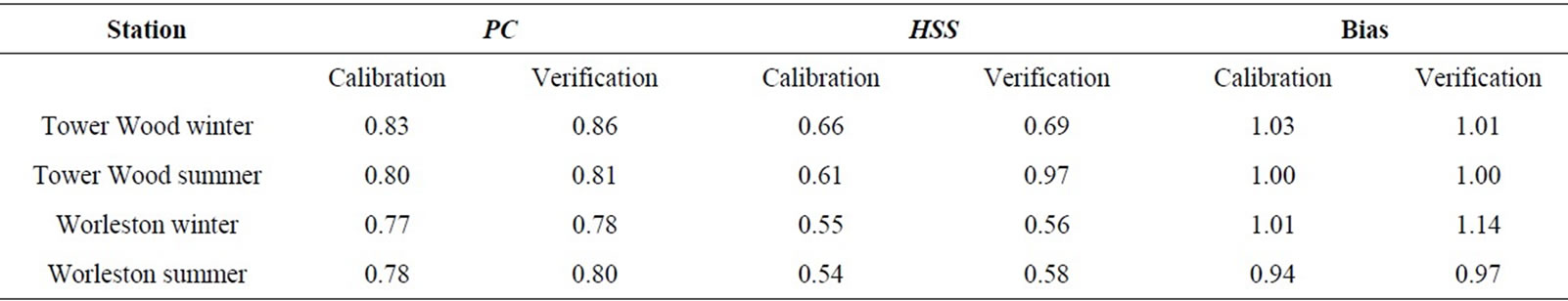
Table 4. Percent correct (PC), Heidke skill scores (HSS) and Bias for the winter-summer rainfall occurrence models for both calibration (1961–1987) and verification (1988–2001) periods for Hybrid model.
Figures 2-5 show the inter-annual variability between the observed and simulated rainfall series for winter and summer for the period 1961-2001(calibration and verification periods) for the two stations. The average yearly values appear to have been adequately captured by the GLM-
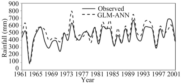
Figure 2. Inter-annual variability for observed and modeled winter rainfall for Tower Wood during calibration and verification periods (1961-2001).
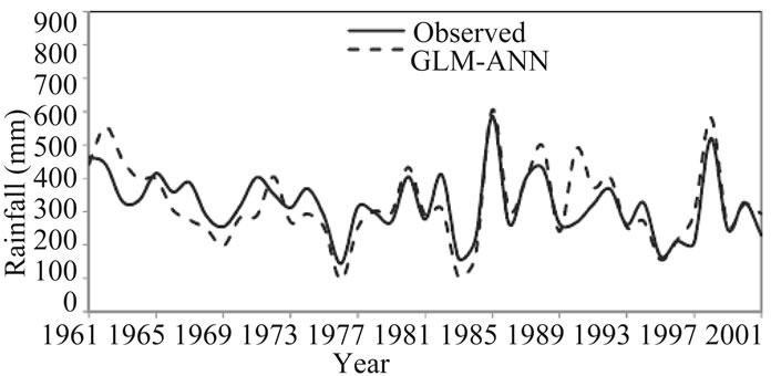
Figure 3. Inter-annual variability for observed and modeled summer rainfall for Tower Wood during calibration and verification periods (1961-2001).
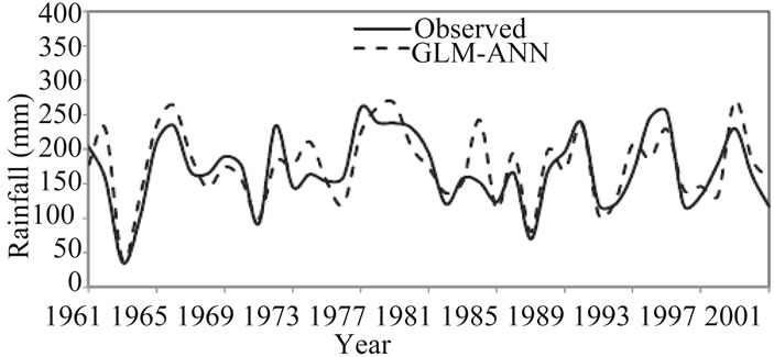
Figure 4. Inter-annual variability for observed and modeled winter rainfall for Worleston during calibration and verification periods (1961-2001).
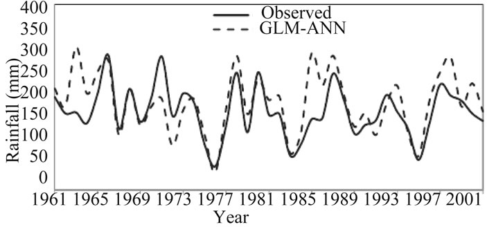
Figure 5. Inter-annual variability for observed and modeled summer rainfall for Worleston during calibration and verification periods (1961-2001).
ANN model. Therefore, these results demonstrate that the hybrid GLM-ANN model used here is accurate in reproducing the observed rainfall which considered to be the most important requirement when assessing climate impacts on a hydrological system.
Another diagnostic test for reproduction of rainfall values, is a plot of quantiles of observed versus simulated rainfall values as can be seen in Figures 6-7. The figures show the quantile-quantile plot for years1961-2001 (calibration and verification period). At both stations, it can be observed that the GLM-ANN model follows the 45˚ line for all rainfall values in winter and summer, suggesting that the GLM-ANN model is closer to the observed rainfall distribution and that winter extreme rainfall is well represented by the GLM-ANN. For the summer, there are some outliers for extreme amounts in the GLM-ANN outputs; however, the model has still shown good overall performance.
The winter is considered the wettest season and the summer is the drier one. So the aim of this paper is to explore the extreme pattern of rainfall under these two conditions. Moreover, using the high and low scenarios of greenhouse emissions would lead for assessing the climate condition at worst conditions (highest and lowest) for these seasons. However most studies undertaken used the medium scenario and few considered the above scenarios.
5.2. Quantifying the Changes in Future Rainfall Extremes
Figure 8 shows an example of threshold selection using parameter stability and the mean residual plot described earlier. The plot shows that a threshold of 11 mm for Tower Wood summer (e.g. under scenario A1FI for future period 2050s) is good choice for the Peak-overthreshold model with GPD, as values of the shape and scale parameter tend to be constant from 11 mm.
Performance of fitting GPD appears in Figure 9 (example is given for Tower Wood summer in 2050s) which demonstrates that the model is well represented by the extremes in terms of probability, quantile, return level and PDF plots.
Following fitting of the GPD to the extracted POT extreme values series, return levels (quantiles) for the base period (1961-1990) and future periods (the 20s, 50s and 80s) have been calculated using Equation (11) for specified return periods. Analysis of the obtained quantiles yields significant changes in the intensity and frequency (return period) of the rainfall extremes in the future periods of the 2020s, 2050s and 2080s compared to the base period of 1961-1990, in both studied catchments.
In winter, rainfall in the Windermere catchment is projected to experience an increase in heavy rainfall under the high (A1FI) and low (B1) scenarios, while in the
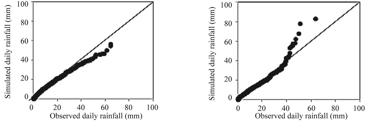
Figure 6. Quantile-Quantile plot of daily rainfall for year 1961-2001 (calibration & verification period) for Tower Wood winter (left) & summer (right).
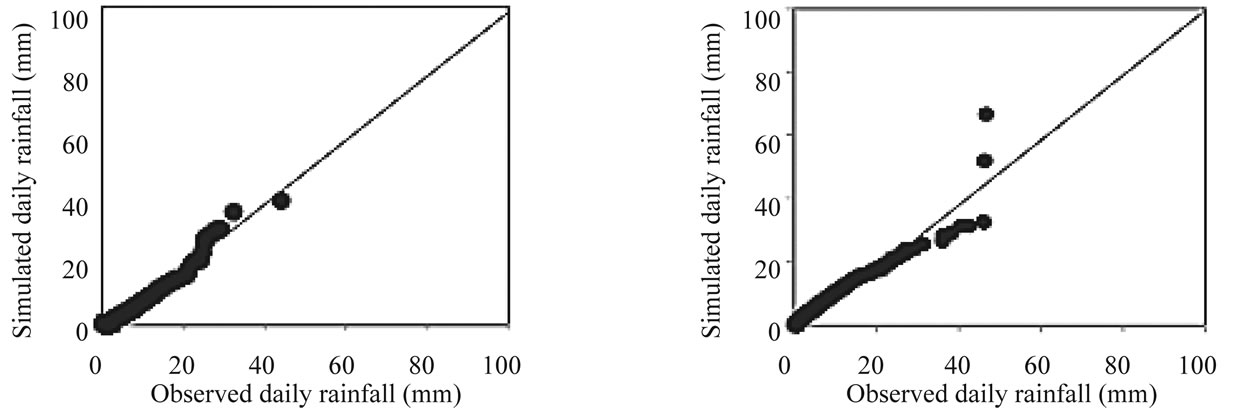
Figure 7. Quantile-Quantile plot of daily rainfall for year 1961-2001(calibration & verification period) for Worleston winter (left) & summer (right).
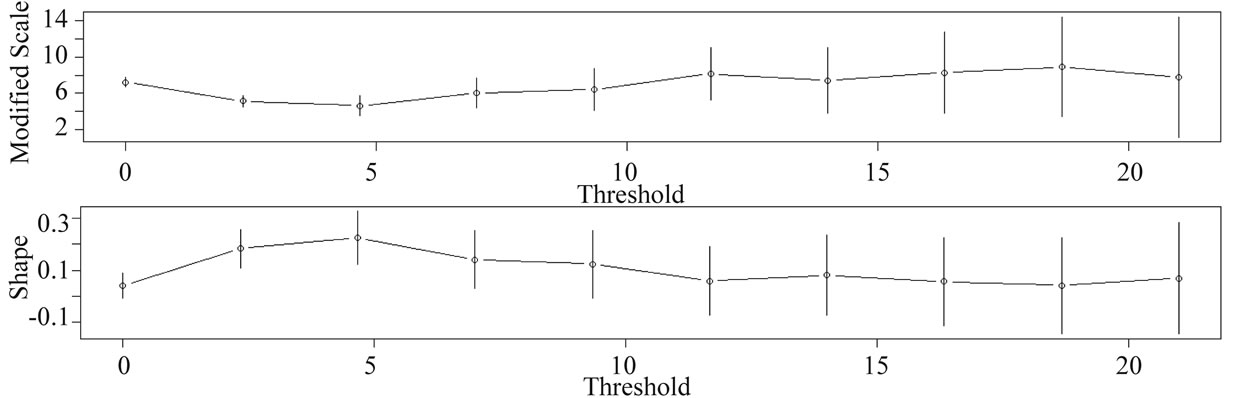
Figure 8. Shape (top) and scale parameter estimated for different thresholds for Tower Wood summer (A1FI, 2050s). Both estimates of shape and scale parameter near constant from 11 mm. Hence, we choose threshold 11 mm.
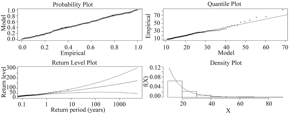
Figure 9. Performance of GPD fitting using rainfall extremes with the selected threshold 11 m for Tower Wood summer (A1FI, 2050s).
Crewe catchment the increase is projected under scenario A1FI only. Sometimes, the increase in winter storms would only be associated with the storms of a high return period of 20 years and thereafter in the 2020s as in the case in the Windermere catchment under scenario B1 (see Figure 10). However, in the 2050s and 2080s, the increase is predicted to be even for storms of low return period (see Figures 10 and 11).
In summer, the Windermere catchment is predicted to have significant increase of extreme rainfall in the 2020s, 2050s and 2080s under the high scenario (A1FI), which is attributed to its location in the wettest region of Northwestern England (Figure 12). However, for the same scenario, the increase in the Crewe rainfall, would only be associated with the 2020s, with a considerable drop in the 2050s and 2080s (see Figure 13). For the low scenario (B1), the two catchments are predicted to suffer from significant reduction in extreme rainfall and that is attributed to the reduction in the greenhouse emissions considered in this scenario, as the assumption inherent in the emission scenario B1 which considers the use of clean energy (see Figures 12 and 13).
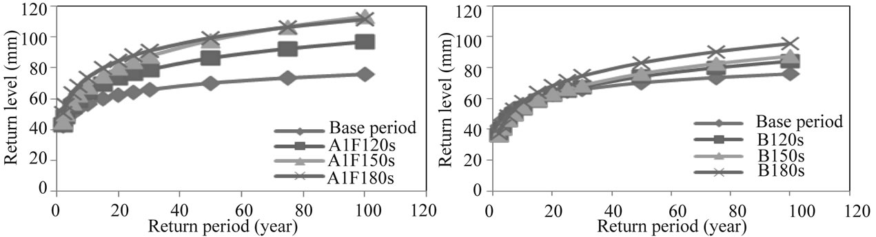
Figure 10. Return level & Return period for Windermere in winter under A1FI & B1 scenario emission.
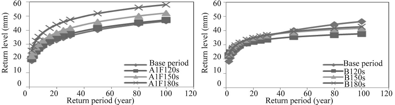
Figure 11. Return level & Return period for Crewe in winter under A1FI & B1 scenario emission.
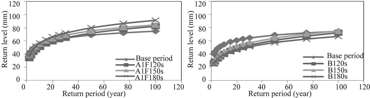
Figure 12. Return level & Return period for Windermere in summer under A1FI & B1 scenario emission.
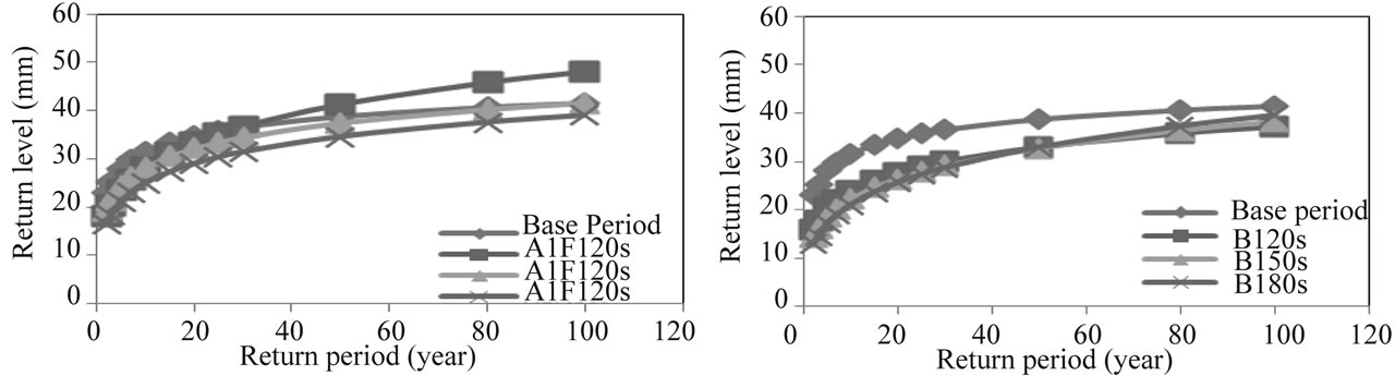
Figure 13. Return level & Return period for Crewe in summer under A1FI & B1 scenario emission.
6. Conclusions
In the present study, downscaling from Global Climate Model (HadCM3), frequency analysis and assessment of future extreme rainfall under scenarios A1FI and B1 for two urban catchments in the Northwest region of England has been addressed.
For the downscaling part, screening for suitable predictors from NCEP data is carried out to build the rainfall occurrence and amount models. The downscaling model used is the hybrid Generalised Linear Model and Artificial Neural Network modeling approach (GLM-ANN).
Frequency analysis to establish the relationship between extreme rainfall and its frequency of occurrence is then carried out on the observed and downscaled rainfall time series. The approach used in the frequency analysis is the combined Peak-over-Threshold Generalised Pareto Distribution (POT_GPD) model.
Changes in the frequency and magnitude of extreme rainfall for winter and summer seasons, under scenarios A1FI and B1, for the considered standard base period (1961-1990) and selected future periods, have then been discussed and assessed.
The study found that increase in frequency of extreme rainfall depends on its own return period, season of the year, the future period considered and the emission scenario under which it was predicted. In the winter season both studied catchments are predicted to experience increase in extremes intensity under scenario A1FI. Under scenario B1, only Windermere would experience an increase in extremes intensity. In both studied catchments, summer extreme rainfalls are projected to increase in frequency under the high emission scenario (A1FI), however the increase for Worleston is only predicted to be in the 2020s. The two catchments are predicted to suffer from a decrease in frequency of extreme rainfall under the low emission scenario (B1) during the summer seasons.
REFERENCES
- G. A. Tank, F. Zwiers and X. Zhang, “Guidelines on Analysis of Extremes in a Changing Climate in Support of Informed Decisions for Adaptation,” WMO, Geneva, 2009.
- IPCC, “Climate Change: The Physical Science Basis, Summary for Policymakers and Contribution of Working Group I to the Fourth Assessment Report of the Intergovernmental Panel on Climate Change,” IPCC Secretariat, Geneva, 2007.
- T. Hailegeorgis and D. Burn, “Uncertainity Assessment of the Impacts of Climate Change on Extreme Precipitation Events,” Canadian Foundation for Climate and Atmospheric Sciences Project, WMO, 2009.
- H. J. Fowler, D. Cooley, S. R. Sain and M. Thurston, “Detection Change in UK Extreme Precipitation Using Results from the Climateprediction.Net BBC Climate Change Experiment,” Springer Science, Vol. 13, No. 2, 2010, pp. 241-267. doi:10.1007/s10687-010-0101-y
- T. J. Osborn and M. Hulme, “Evidence for Trends in Heavy Rainfall Events over the UK,” The Royal Society, Vol. 360, No. 1796, 2002, pp. 1313-1325.
- M. Sanderson, “Changes in the Frequency of Extreme Rainfall Events for Selected Towns and Cities,” Ofwat, UK, 2010.
- B. Yarnal, A. Comrie, B. Frakes and D. Brown, “Developments and Prospects in Synoptic Climatology,” International Journal of Climatology, Vol. 21, No. 15, 2001, pp. 1923-1950.
- H. J. Fowler, S. Blenkinsop and C. Tebaldi, “Linking Climate Change Modelling to Impacts Studies: Recent Advances in Downscaling Techniques for Ydrological Modelling,” International Journal of Climatology, Vol. 27, No. 12, 2007, pp. 1547-1578. doi:10.1002/joc.1556
- R. Huth, “Statistical Downscaling in Central Europe: Evaluation of Methods and Potential Predictors,” Climate Research, Vol. 13, No. 2, 1999, pp. 91-101. doi:10.3354/cr013091
- C. Harpham and R. L. Wilby, “Multisite-Downscaling of Heavy Daily Precipitation Occurrence and Amounts,” Journal of Hydrology, Vol. 312, No. 1-4, 2005, pp. 235- 255.
- P. McCullagh and J. Nelder, “Generalized Linear Models,” 2nd Edition, Chapman & Hall, London, 1989.
- R. E. Chandler and H. S. Wheater, “Analysis of Rainfall Variability Using Generalized Linear Models—A Case Study from the West of Ireland,” Water Resources Research, Vol. 38, No. 10, 2002, p. 1192. doi:10.1029/2001WR000906
- K. P. Chun, “Statistical Downscaling of Climate Model Outputs for Hydrological Extremes,” Ph.D. Dissertation, Imperial College, London, 2010.
- D. Wilks, “Statistical Methods in Atmospheric Sciences,” Academic Press Limited, London, 1995.
- Weather Forecasting On-Line, “Verification Measures,” 2010. http://www.wxonline.info/topics/verif2.html
- D. Yadav, N. R. Naresh and V. Sharma, “Stream Flow Forecasting Using Levenberg-Marquardt Algorithm Approach,” International Journal of Water Resources and Environmental Engineering, Vol. 3, No. 1, 2010, pp. 30- 40.
- D. Maraun, F. Wetterhall, A. M. Ireson, R. E. Chander, E. J. Kendon, M. Widmann, S. Brienen, H. W. Rust, T. Sauter, M. Themebl, V. K. C. Venema, K. P. Chun, C. M. Goodess, R. G. Jones, C. Onof, M. Vrac and I. ThieleEich, “Precipitation Downscaling under Climate Change: Recent Developments to Bridge the Gab between Dynamical Models and the End User,” Reviews of Geophysics, Vol. 48, RG3003, 2010, 34 p.
- J. Pickands, “Statistical Inference Using Extreme Order Statistics,” The Annals of Statistics, Vol. 3, No. 1, 1975, pp. 119-131.
- J. Palutikof, T. Holt, B. Brabson and D. Lister, “Method of Calculate Extremes in Climate Change Studies,” University of East Anglia, Norwich, 2003.
- C. White1, A. Sanabria, S. Corney, M. Grose, G. Holz, J. Bennett1, R. Cechet and. N. Bindoff1, “Modelling Extreme Events in a Changing Climate using Regional Dynamically-Downscaled Climate Projections,” International Environmental Modelling and Software Society, 2010.
- L. Fawcett and D. Walshaw, “Modelling Environmental Extremes,” Short Course for the 19th Annual Conference of the International Environmetrics Society, Kelowna, 8-13 June, 2008.
- S. Coles, “An Introduction to Statistical Modelling of Extreme Values,” Springer Series in Statistic, London, 2001.
- A. C. Davison, “Modelling Excesses over High Thresholds, with an Application in Statistical Extremes and Applications,” In: J. Tiago de Oliveira, Dordrecht, Ed., Statistical Extremes and Applications, D. Reidel, Dordrecht, 1984, pp. 461-482.
- W. Ledermann, E. Lioyd, S. Vajda and C. Alexander, “Handbook of Application Mathematics,” Supplement, Wiley-Interscience, Chichester, Vol. 7, 1990, p. 479,
- J. R. M. Hosking and J. R .Wallis, “Parameter and Quantile Estimation for the Generalized Pareto Distribution,” Technometric, Vol. 29, No. 3, 1987, pp. 339-349. doi:10.2307/1269343
- R. L. Smith, “Maximum Likelihood Estimation in a Class of Non-Regular Cases,” Biometrika, Vol. 72, No. 1, 1985, pp. 67-90. doi:10.1093/biomet/72.1.67
- E. Gilleland, R. Katz and G. Young, “Extremes Toolkit (Extremes), Weather and Climate Applications of Extreme Value Statistics,” 2005. http://www.assessment.ucar.edu/toolkit/
- D. Conway, R. Wilby and P. D. Jones, “Precipitation and Air Flow Indices over the British Isles,” Climate Research, Vol. 7, No. 2, 1996, pp.169-183. doi:10.3354/cr007169