Open Journal of Modern Hydrology
Vol.2 No.2(2012), Article ID:18559,12 pages DOI:10.4236/ojmh.2012.22005
Assessing the Efficacy of Two Indirect Methods for Quantifying Canopy Variables Associated with the Interception Loss of Rainfall in Temperate Hardwood Forests
![]()
1School of Forest Resources and Environmental Science, Michigan Technological University, Houghton, USA; 2Yeongsan River Environment Research Center, National Institute of Environmental Research, Ministry of Environment, Gwangju, Korea.
Email: tgpypker@mtu.edu
Received December 2nd, 2011; revised January 10th, 2012; accepted February 21st, 2012
Keywords: canopy water storage; evaporation; Direct throughfall; Gash model; sugar maple; mean method; IS method
ABSTRACT
Forest canopy water storage (S), direct throughfall fraction (p) and mean evaporation rate to mean rainfall intensity ratio ( ) vary between storms and seasonally. Typically, researchers only quantify the mean growing and dormant season values of S, p and
  for deciduous forests, thereby ignoring seasonal changes S, p and
 . Past researchers adapted the mean method, which is usually used to estimate S, p and
  on an annual or seasonal basis, to estimate the same canopy variables on a per storm basis (individual storm (IS) method). The disadvantage of the IS method is that it requires more expensive equipment and the calculation of the canopy variables is more labor intensive relative to the mean method. The goal of this study was to explore the use of the IS method for northern hardwood forests and to determine whether estimates of S, p and
  derived by the IS method produce more accurate estimates of rainfall interception loss (In) using the Gash model relative to estimates derived by the mean method. The IS method estimated that S increased from approximately 0.11 mm in the early spring to 1.2 mm in the summer and then declined to 0.24 mm after fall senescence. Direct throughfall decreased from 0.4 in the early spring to 0.11 in the summer, and then increased to 0.4 after leaf senescence. When measurement period estimates of p, S and
  derived by the IS and mean methods were applied to the Gash model, the modeled estimates of In differed from the measured values by 14.0 mm and 1.3 mm, respectively. Therefore, because the mean method provided more accurate estimates of In, the extra effort and expense required by the IS method is not advantageous for studies in northern hardwood forests that only need to model annual or seasonal estimates of In.
1. Introduction
In forested ecosystems, the rainfall interception loss (In: Gross precipitation minus net precipitation (mm)) can be seasonally variable [1] and can account for about 10% - 40% of a forest’s annual gross precipitation [2]. For this reason, researchers have developed empirical models to estimate rainfall interception loss by a forest [e.g. 3,4-8]. These models are typically parameterized using mean yearly or mean seasonal estimates of canopy water storage (S), direct throughfall fraction (p), canopy saturation point (Ps) and mean ratio of evaporation to rainfall intensity ( ) (for precise definitions of the variables see Section 2.2). While these empirical models will produce accurate estimates of In on an annual basis, the use of mean annual or mean seasonal canopy variables does not demonstrate how these variables and subsequent hydrologic processes will change from storm to storm.
Methods exist for quantifying changes in canopy variables. For example, some researchers have used the attenuation of microwaves [9,10] or gamma rays [11] to quantify canopy parameters. These methods can estimate seasonal changes in canopy variables, but they are very expensive and not readily available. Link et al. [12] proposed a less expensive method that allows for estimates of p, S and  for individual storm events (IS method). This method applies the mean method [10] to individual storms by relating the cumulative measurement of net precipitation (Pn) by an array of tipping bucket rain gauges that are randomly distributed under a forest, to the cumulative measurement of cumulative gross precipitation (PG). By finding the inflection point between the PG and Pn, it was possible to determine seasonal changes in p, S and
  of an old-growth Douglas-fir forest. Using this method, Link et al. [12] reported that S decreased slightly after seasonal leaf-drop in the fall. More recently, Herbst et al. [13] demonstrated that the method could track changes in p, S and
  from storm to storm in a deciduous forest. Furthermore, Herbst et al. [13] applied the variables to the Gash model [14] and found the IS method produced accurate results.
To apply the IS method one requires large number of relatively expensive tipping bucket rain gauges and increased computer computations. In contrast, the original mean method requires simple throughfall collectors that quantify gross precipitation and net precipitation on a storm by storm basis or a weekly basis to estimate p, S and  on an annual or seasonal basis. The goal of this study is 1) to confirm that the IS method is appropriate for temperate hardwood forests 2) determine if the extra effort required for the IS method provides better estimates of In using the commonly used Gash model [3] relative to the canopy variables derived via the original mean method.
2. Materials and Methods
2.1. Study Site
The study area was located in the Huron Mountains in the Upper Peninsula of Michigan, USA (46.9˚N, 87.4˚W). The forest is dominated by mature sugar maple (Acer Saccharum Marsh) with smaller components of tree basal area occupied by ironwood (Ostrya virginiana (P. Mill.) K. Koch) and yellow birch (Betula Alleghaniensis Britton) (Table 1). Canopy height was between 25 m and 30 m. The region has cold, snowy winters and warm, wet summers with a mean precipitation from May through October of approximately 514 mm [15]. The soil is comprised of ~80% sand, ~15% - 20% silt and 3% - 5% clay (Lilleskov, personal communication).
2.2. Terminology
Variables used in this paper follow the definitions outlined by Gash [14]. All models assume that there is a wet up period that ends when the cumulative gross precipitation (PG) is equal to the canopy saturation point (Ps) (mm). The canopy storage capacity (S) is defined as the
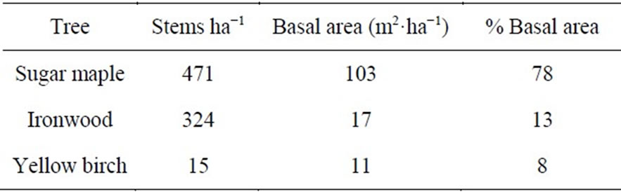
Table 1. The stem density, basal area and percent basal area of the three dominant tree species at the study site.
quantity of rainfall (mm) found on surface of the canopy and trunks, if evaporation was zero and rainfall and throughfall have ceased [14]. The direct throughfall fraction (p) is defined as the proportion (unitless) of the rainfall that falls directly to the forest floor. The ratio of the mean evaporation ( ) rate (mm·h−1) to mean rainfall rate (
 ) (mm·h−1) was estimated for periods when PG is greater than Ps. Rainfall interception loss (In) is defined as the difference between the gross precipitation (PG) that entered the top of the forest canopy minus the net precipitation (Pn) that exited the bottom of the forest canopy.
2.3. Measurement of Gross Precipitation and Net Precipitation
From 1 May to 6 November 2007, PG and Pn were measured using tipping bucket rain gauges (RG3-M, Onset Computer Corp., Bourne, MA). The tipping buckets were placed approximately 1 m above the ground and monitored using individual dataloggers that recorded the time of each tip (HOBO Pendant event, Onset Computer Corp.). Each tipping bucket rain gauge has a diameter of 15.2 cm and a resolution of 0.2 mm. Two tipping bucket rain gauges were placed in a clearing adjacent to the forest to measure PG (angle from tipping bucket to nearest tree top < 45˚). Twenty tipping bucket rain gauges were placed randomly along a 200 m transect in one of four 30 m by 30 m plots (n = 5 per plot) to measure Pn. Placing the array across the range of variability [16,17] and relocating the collectors on a regular basis (every six weeks) reduces errors in the throughfall estimates by increasing the number of sampling points in the plot [18,19]. We excluded four storm events (DOY 170, 241, 279 and 281) from the analysis because the rainfall intensity exceeded the capacity of the tipping bucket rain gauges. These rainfall events were significant, but cannot be used in the comparison as the accuracy of the tipping buckets is in question. It should be recognized that the loss of this data limits the comparison of modeling methods to storms with rainfall intensities less than 10 mm·h−1.
2.4. Stemflow
Stemflow measurements were made on 20 trees (16 sugar maple and 4 ironwood trees) from 1 June to 30 September 2007. Measurements were made by cutting a 2 cm diameter garden hose in half longitudinally and attaching it in a spiral fashion around the stem of the trees using a staple gun and silicone caulking. The hose encircled the circumference of the tree twice before being fed into a 20 L plastic container. The contents of the buckets were monitored on a weekly or biweekly basis.
2.5. Calculation of Canopy Variables
The mean and IS methods were used to estimate S, p, Ps and  from 1 May to 6 November 2007. For accuracy, bucket type models such as the mean and IS methods assume that: 1) the entire canopy saturates simultaneously during the storm event; and 2) the canopy is dry prior to a storm event.
With the mean method, S, p and  were estimated by creating two regression lines (R1 and R2) that related below-canopy net precipitation during the storm (Pn (mm)) to the gross precipitation (PG (mm)) [10]. The first regression line (R1) was fit to all the storm events where PG was insufficient to saturate the canopy. The second regression line (R2) was fit to all storm events where PG was sufficient to saturate the canopy. The slope of each regression line was determined by an iterative least squares fitting procedure [12,13]. When using the mean method, the slope of R1 provides the estimate of p; one minus the slope of R2 provides an estimate of
 . The value of PG at the intersection point of R1 and R2 provides an estimate of the canopy saturation point (Ps); and the difference between PG and Pn at the intersection point of R1 and R2 provides an estimate of S.
Values of S, p, and  were calculated on a “per storm” basis using the IS method as described in Link et al. [12]. To apply the IS method, we required a minimum of 5 mm of rainfall, a minimum of 8 h between rainfall events [20], no more than 1 h of rainless periods during rainfall events less than 4 h and no more than 2 h of rainless periods during storms greater than 4 h [13,21]. A minimum rainfall amount is needed for the IS method because a linear regression is applied to the relationship between cumulative gross (PG) and cumulative net precipitation (Pn). Extended periods with no rainfall will result in partial canopy drying. This affects the estimates of
  and S. Under these criteria, extended periods of drying are limited, but not entirely eliminated. Lastly, if each rain gauge has an error of less than 10%, the use of an inflection point reduces the error in S to approximately 10% [13].
Canopy variables were calculated for 10 rainfall events from 1 May to 6 November 2011. Similar to the mean method, the IS method partitions each rainfall event into two discrete periods; preand postcanopy saturation. The IS method can be advantageous because it calculates the canopy variables on a per storm basis using equations (1)-(4). Equation (1) quantifies the amount of rainfall passing through the forest canopy prior to canopy saturation, equation (2) quantifies Pn for the period post saturation, equation (3) quantifies S and equation (4) quantifies the amount of rainfall lost to evaporation during wet-up. A complete description can be found in Link et al. [12].
Linear regressions was create for both the preand postcanopy saturation periods that related the two minute totals of Pn to PG. The slope of each regression line was determined by an iterative regression method [12,13]. Prior to canopy saturation, the relationship between Pn and PG was calculated as:
 (1)
(1)
where p is the proportion of rainfall that passes through the canopy prior to canopy saturation (Figure 1).
Prior to saturation, it is assumed that the intercepted water will either remain in the canopy as stored water or evaporate. Following saturation, intercepted rainfall will either drip to the forest floor or evaporate (Figure 1). Post-saturation throughfall was computed using:
 (2)
(2)
where  is the ratio of evaporation to rainfall intensity and Ps is the canopy saturation point (mm). Direct throughfall fraction was calculated using the slope of Equation (1) and
  was calculated as one minus the slope of the second line (Figure 1). S is then computed by:
 (3)
(3)
where IW is the rainfall that is evaporated during canopy wet-up. Iw was estimated by:
 (4)
(4)
The use of Iw can result in an overestimation of evaporation [22] because it assumes the canopy is fully saturated during wet-up. During storm events where the canopy requires a long period to saturate, the canopy can be partially saturated for extended periods. This will reduce the evaporation from the forest because only a portion of the canopy can contribute to evaporation. For this reason, S was estimated with Iw(Sw) and ignoring Iw(Swo) in Equation (3) and the difference was compared.
2.6. Evaluation of the Gash Model in a Northern Hardwood Forest
The Gash model is a powerful tool for estimating In because of its simple requirements of S, p and  [14].
[14].
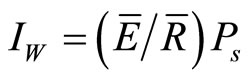
Figure 1. The IS method estimates canopy water storage (S), direct throughfall fraction (p), ratio mean of evaporation rate to mean rainfall intensity ( ) and canopy saturation point (Ps) by relating the cumulative gross precipitation to the cumulative net precipitation for storms during the full leaf out (a) and transition (b) periods. Here the slope of the first line represents p (0.23 and 0.30 for (a) and (b), respectively) and 1 minus the slope of the second line equals
  (0.06 and 0.28 (a) and (b), respectively) (see Section 2.5). Please note that the different storm sizes results in different scales on the graph axes of (a) and (b).
The Gash model is the most common rainfall intercepttion model used in interception studies in North America [23]. In short, the Gash model quantifies In for three phases of a rainfall event; pre-saturation, saturation and the drying of the forest canopy. The model assumes the canopy can store an amount of water equivalent to S. After that quantity of water is stored, the subsequent rainfall passes through the canopy as drip or is lost as evaporation. After the rainfall ceases, the water remaining in the canopy is subsequently evaporated back to the atmosphere. A complete description is provided by Gash et al. [14]. For this study, the Gash model was extremely useful because meteorological data was limited. The model is, however, limited by the following assumptions outlined by Gash [3]: 1) rainfall is represented by a series of discrete storms separated by periods long enough to allow the canopy to completely dry; 2) the meteorological conditions are constant throughout the storm; and 3) there is no drip from the canopy during wet-up. Clearly, assumptions 2 and 3 are frequently violated during a storm as meteorological conditions such as wind speed, rainfall intensity and vapor pressure deficit can change through the storm and wind speeds may vary and shake the canopy causing drip during wet-up. Yet, the Gash model has proved to be very robust in predicting annual rainfall interception loss [14]. The following is the Gash model for sparse canopies [14]. The interception (Ic) during m small storms that were insufficient to saturate the canopy is described by:
 (5)
(5)
where c represents the canopy cover. The canopy cover was assumed to equal 1 – p [13,14]. The amount of interception for n storms sufficient to saturate the canopy (i.e. ³the amount of rainfall to saturate the canopy—Ps) is calculated as the amount of water lost during wet up (Iw), the evaporation after canopy saturation, but prior to rainfall ceasing (IS) and the evaporation after the storm ceases (Ia). These interception variables are calculated as:
 (6)
(6)
 (7)
(7)
 (8)
(8)
We parameterized the Gash model using estimates of p, Sw, Ps, and  from the IS and mean method. Both the IS and mean methods produced two different estimates of p, Sw, Ps, and
  for use in the Gash model. The first estimates from the IS and mean methods produced an estimate of canopy variables for the entire measurement period (1 May to 6 November) and the second estimate produced seasonal estimate that divided the measurement period into periods with full leaf out (25 June to 10 September 2007) and without full leaf out (defined for the rest of the paper as the “transition periods”) (1 May to 20 June and 11 September to 6 November 2007). The IS method produced a measurement period mean of p = 0.17, Sw = 0.79 mm, Ps = 1.16 mm and
  = 0.14 using every other storm as estimated by the IS method (Table 2, starting with storm 7). Using the same storms, the IS method estimated p, Sw, Ps, and
  during full leaf out (p = 0.23; Sw = 1.21; Ps = 1.69;
  = 0.06) and transition periods (p = 0.16; Sw = 0.68; Ps = 1.03;
  = 0.17). The mean method produced a measurement period mean of p = 0.20; Sw = 0.9; Ps = 1.49;
  = 0.19. Finally, the mean method estimated p, Sw, Ps, and
  during full leaf out to be p = 0.18; Sw = 1.92; Ps = 2.49; and
  = 0.05 and during the transition periods to be p = 0.3; Sw = 0.9; Ps = 1.69; and
  = 0.17. When applying the Gash model, we excluded storms that provided the estimates of p, Sw, Ps, and
  from the IS method. Therefore, the measured In for the storms used in the modeling exercise totaled 77.5 mm. We used Sw instead of Swo, because the inclusion of evaporation during wet-up should result in more accurate estimates of S. However, the differences between Sw and Swo were not very large because sampling protocol for the IS method only used storms where gaps in rainfall were less than 2 hours. This resulted in Sw and Swo producing similar estimates of S.
3. Results and Discussion
3.1. Gross Precipitation (PG), Net Precipitation (Pn) and Interception Loss
From 1 May to 6 November 2007, PG and Pn for measured storms totaled 343 mm and 247 mm, respectively (Table 2). In late summer and early fall, there were several high intensity rainfall events (ranging between 60 and 240 mm·h−1) that exceeded the capacity of the tipping buckets for short periods of time (>20 minutes). The storms on 18 June, 28 August and the 2, 5 and 7 of October (n = 5) were not included in Table 2 nor were they used in the IS method or the Gash model because their inclusion could result in inaccurate estimates. While the exclusion of these storms precludes an accurate seasonal estimate of In for the stand, it does not preclude a comparison between the IS method and the mean method for the available storms where rainfall intensities did not exceed 10 mm·h−1. When the estimated values from these five storms are included in the dataset, the site is estimated to have received approximately 590 mm of rainfall during the study period (data not shown); 70 mm to 80 mm more than the long term mean of 514 mm [15]. From 1 June to 27 August, the site received approximately 91 mm of rainfall, far short of the typical 194 mm [15]. The site received a normal amount of rainfall over the study period because precipitation from 28 August to 6 November
(433 mm) was greater than the long term mean (162 mm) [15].
Mean rainfall intensity for each storm was fairly constant throughout the measurement period, ranging from 0.63 to 5.3 mm·h−1 (Figure 2). With the exception of 6 storm events, mean rainfall intensity was below 2 mm·h−1. There is no significant linear relationship between date and rainfall intensity (p-value > 0.85). Past research suggests that S is correlated to changes in rainfall intensity [24,25], but the effect is still under debate [26-28].
For the storms used in this study, the forest lost 95 mm, or 28.6% of PG to In (Table 2). Typically, In ranges between 10 and 35% in broadleaf forests [e.g. 8,29-31]. When compared to measurements in other regional hardwood forests, In in this study was higher than the 10 to 15% reported by Helvey and Patric [30] for northern hardwoods, but is closer to the 20% reported by CarlyleMoses and Price [29] for oak dominated stands in southern Ontario, Canada. A closed canopied forest can experience greater In if rainfall is spread out over many small storms instead of one large storm that has a low . For example, Horton [32] reported that for storms greater than 25 mm, 20% of the rainfall was lost to evaporation, whereas 30% of rainfall was lost during storms events between 2.5 and 7.6 mm. The mean rainfall event at our study site was less than 7 mm and interception loss ranged from 100% for very small storms to 8% for larger storms (Table 2).
The accuracy of the 20 tipping buckets varied according to storm size (Figure 3). For storms where PG was <5 mm, the 95% confidence interval was typically between 4 to 60% of Pn. For very small storms events (<0.8 mm), three of the 95% confidence intervals exceeded 80% of Pn (for clarity, two are not shown on Figure 3 because they exceeded 100%). The high variability of Pn at low storm sizes is common [18]. For storms where the IS method was applied (PG > 5mm), the 95% confidence intervals were much smaller, with the range typically being within 10% of Pn. Power analysis predicts that for

Figure 2. Mean rainfall intensity for individual storm events from 1 May to 6 November 2007.
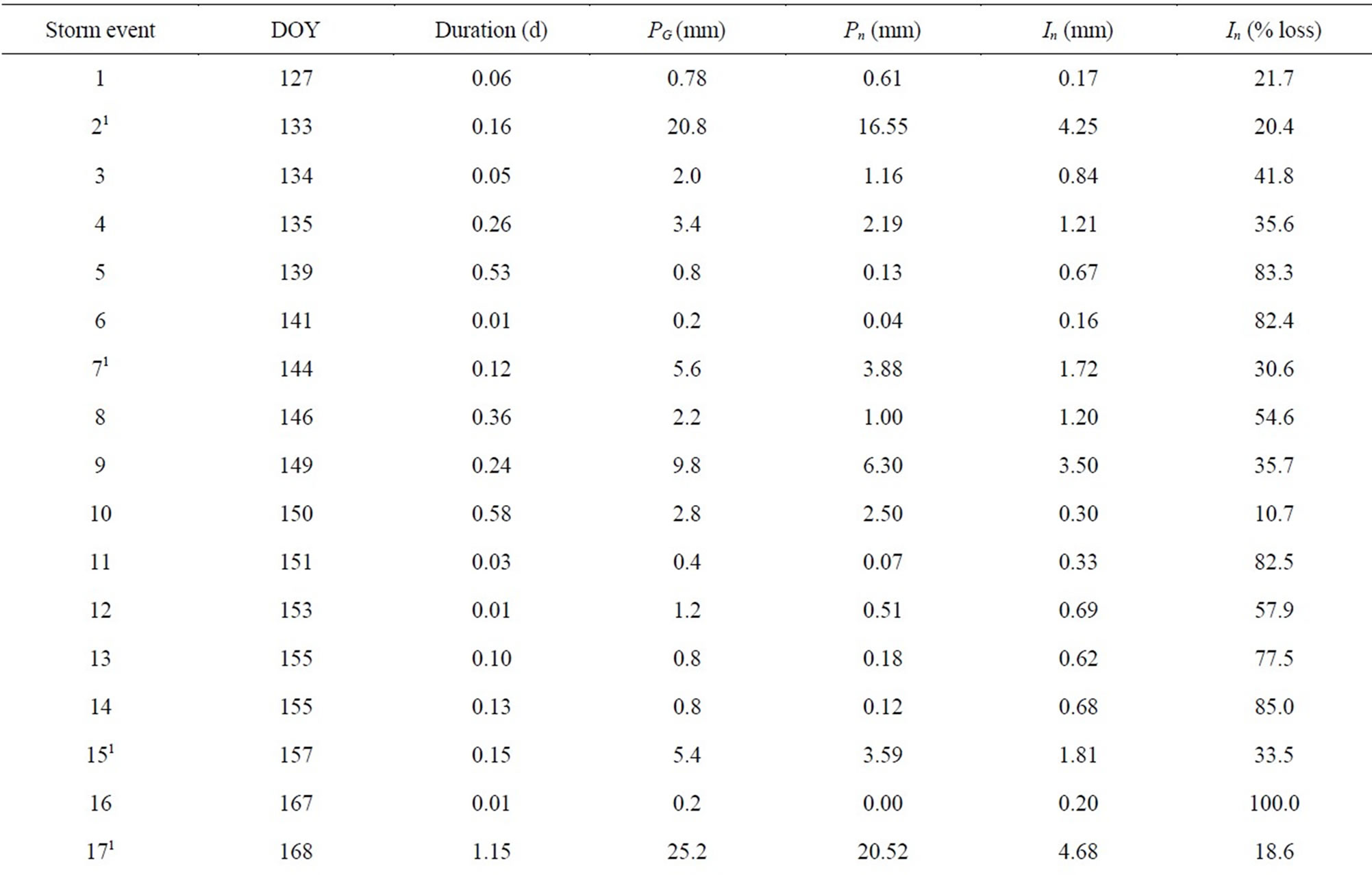
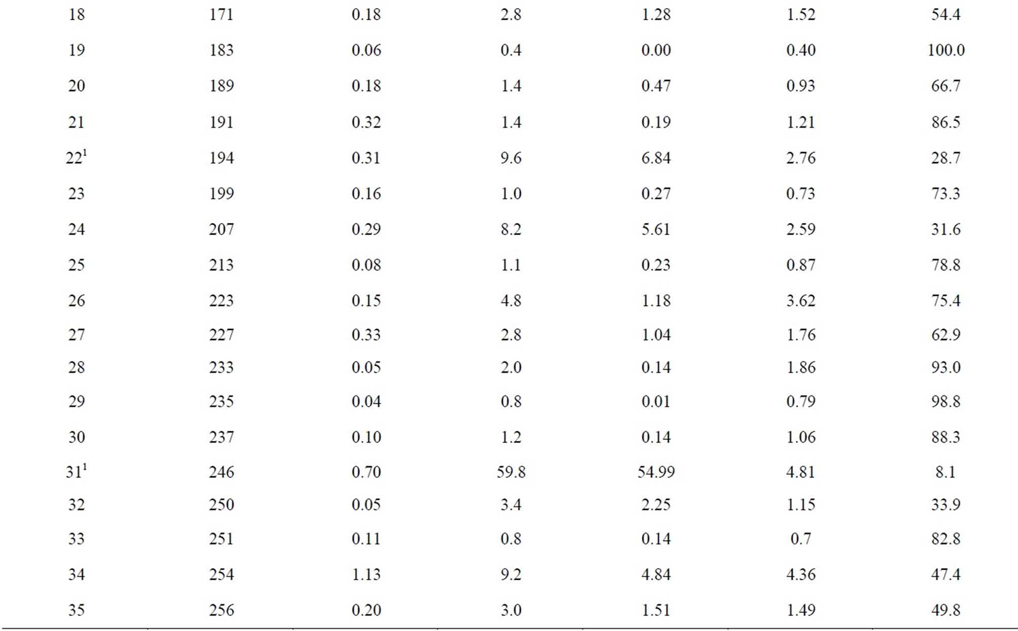

Table 2. The gross precipitation (PG), net precipitation (Pn), total interception loss (In) and percent In, and mean evaporation rate to mean precipitation rate ( ) for storm events from 1 May to 6 November 2007.
Figure 3. Relationship between gross precipitation and the 95% percent confidence interval of net precipitation (presented as a percent of net precipitation). Rainfall events that are greater than 5 mm are to the right of the dashed line.
storms greater than 5 mm, one would need 5 to 90 throughfall collectors to estimate within 5% of the actual Pn. However, a sample size of less than 16 tipping bucket is needed to estimate within 10% of the actual Pn.
3.2. Canopy Variables
Canopy water storage varied seasonally. When the IS method ignored evaporation during wet-up, Swo increased from 0.15 mm (13 May 2007) to greater than 1.3 mm during full leaf-out (Figure 4). Following senescence, Swo decreased to 0.4 mm (Oct 18) (Figure 4). When evaporation is accounted for during wet-up, Sw ranged from 0.11 mm during the transition period to 1.2 mm during full leaf-out. When evaporation during wet-up was excluded from the analysis, the estimates of Swo were usually only slightly larger than Sw, with the difference often ranging between 0.04 mm to 0.3 mm. The differences between the two estimates are limited because we only included storms that had short periods when rainfall ceased (see section 2.5). This restriction removed storms were the wet-up period was long because of intermittent
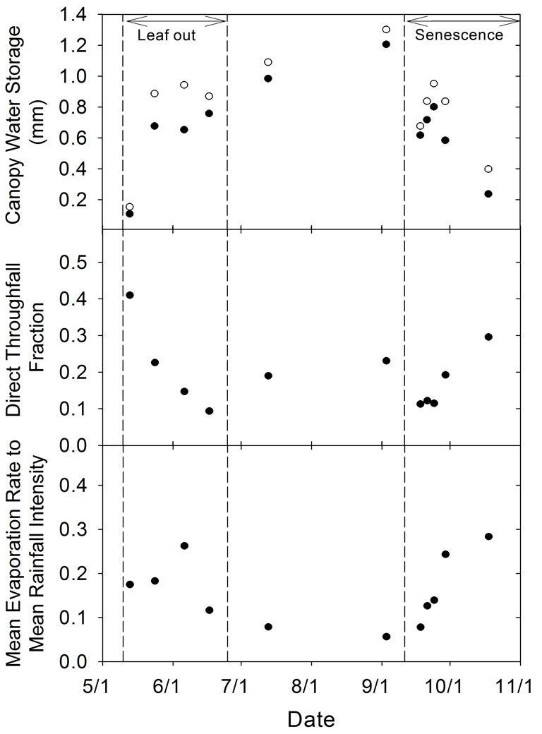
Figure 4. Seasonal changes in the canopy water storage with (Sw, closed circles) and without (Swo, open circles) evaporation during wet-up, direct throughfall fraction (p) and mean evaporation rate to mean rainfall intensity ratio ( ) as estimated by the IS method (see Section 2.5). Measurements were made in a sugar maple dominated stand from 1 May to 6 November 2007. The vertical dashed lines represent the period of full leaf out and senescence in the stand.
rainfall.
For northern hardwood or mixed northern hardwood forests, past research estimated S to range between 0.2 and 2.0 mm [1,8,29,33]. However, past research only reports a mean value for the entire year or for the leafless and full leaf out periods. At our study site, Sw averaged 1.09 mm during full leaf out. In the spring and fall transition periods, Sw was variable, ranging from 0.1 mm to greater than 0.75 mm. The mean method predicted slightly different values. The mean method estimated S to be 0.89 mm during the transition periods and 1.92 mm during full leaf out. Both estimates are within the range reported by others. However, the IS method is advantageous because it provides evidence for the seasonal change in S and p throughout the growing season [13].
Even without changes in the canopy structure, S will vary with rainfall intensity [24] and changing wind speed [2,34]. Calder et al. [24] hypothesized that increasing rainfall intensity resulted in a decrease in S; and Hörmann et al. [2] found S was influenced by inter-storm variation in windspeed and severity of wind gusts, which shake stored water off leaves/branches. The IS method provides a tool to investigate variation in canopy variables as they relate to changes in canopy structure, rainfall intensity and windspeed. For the dataset in this study, there was not a significant linear relationship between any canopy variable (p, S or ) and mean rainfall intensity (p-values > 0.14, 0.75 and 0.58 for p, S and
 , respectively). The lack of a significant relationship between changes in canopy variables and rainfall intensity is not surprising, as the canopy structure changed throughout much of the measurement period because of changes in leaf area index (LAI). Therefore, changes in canopy structure may be masking the effects of rainfall intensity on changes in canopy variables. To analyze for the effect of rainfall intensity and windspeed, measurements of both LAI and windspeed would be needed throughout the measurement period.
The throughfall fraction (p) ranged from 0.09 to 0.41 over the study period. During the transition periods, p exceeded 0.3, but during the full-leaf out period, p reduced to approximately 0.2 (Figure 4). The mean method produced similar values with p ranging between 0.17 during full leaf out and 0.3 during the transition periods. Direct throughfall fraction has been predicted using the gap fraction of the canopy [35,36]. Hence, one would expect a larger p during the transition periods. However, p does not depend solely on gap size. Other factors such as wind speed will affect the path of the raindrops, thereby affecting the size of p. Hence, changes in micrometeorological variables may have partially caused the high variability of p during the transition periods. Future research that investigates the effect of micrometeorological variables on p is needed. Even with the variability in p, one can see a trend of decreasing p during the summer months and increased p during the early spring and late fall (Figure 4).
The estimates of  ranged from 0.07 to 0.28 with a mean of 0.16 (Figure 4). The mean method produced similar values, with
  ranging from 0.05 during full leaf out to 0.17 during the transition periods. Past work has found
  to range from 0 to 0.4 in temperate forests [1,37]. The value can range widely as changes in wind speed, vapor pressure deficit and rainfall intensity will affect the rate of evaporation following canopy saturation [38]. The IS and mean methods both provided lower values of
  during the summer months relative to the transition periods in spring and fall. Furthermore, when
  is linearly related to changes in rainfall intensity, the slope of the regression line is not significant (slope = −0.01, 95% CI = 0.03, p-value > 0.5). This appears to conflict past work that that has related changes in storage and evaporation to changes in rainfall intensity [39]. This may appear unreasonable as one might expect a greater evaporation during lower rainfall intensities and when the canopy is capable of storing more water.
The increase in  in the fall and spring and the lack of a relationship between rainfall intensity and
  may be reasonable in this forest. The reduction in leaf area alters the canopy structure, thereby making it possible for evaporation to increase. Evaporation from a forest canopy can be highly variable as it depends on wind speed, vapor pressure deficit and canopy aerodynamic resistance [38]. Teklehaimanot et al. [40] reported that an increase in tree density did not linearly increase rainfall interception loss. They reported that the loss in S due to reduced tree coverage was partially compensated by a decline in the aerodynamic resistance of the canopy that increased evaporation. If storms during fall and spring at our research site were accompanied by greater winds, the aerodynamic resistance of the canopy would decrease and evaporative losses would increase. Past work also demonstrates that evaporation rates within the same forest stand can change seasonally [e.g. 13,34]. For example, Herbst et al. [13] reported higher evaporation rates during periods without leaves which they attributed to higher wind speeds, lower aerodynamic resistance and increased evaporation from the forest floor. Therefore, it is possible for the evaporation rates to be greater during the transition periods and for rainfall intensity to not be related to seasonal changes in
 .
.
3.3. Gash Model Estimates
The Gash model produced more accurate estimates of In when using mean method derived estimates of Sw, p,  and Ps, relative to IS method derived estimates. Full leaf out and transition periods estimates (seasonal estimates) of Sw, p,
  and Ps provided by the mean method produced Gash model estimates of In that differed from the measured values by 8.4 mm (Table 3). When mean method estimates from 1 May to 6 November 2007 (annual estimates) were used to provide Sw, p,
  and Ps, the Gash model estimates differed from the measured values by only 1.3 mm. This is similar to past research that demonstrated that using seasonally derived canopy variables improved the estimates of the Gash model [41]. In contrast, seasonally and annually derived estimates of Sw, p,
  and Ps by the IS method resulted in Gash model estimates of In that differed from the measured values by 12.7 mm and 14.0 mm, respectively (Table 3).
The IS method derived estimates of Sw, p,  and Ps caused the Gash model to frequently underestimate In (Figure 5). This may have resulted, in part, because the storms used to estimate S, p,
  and Ps excluded storms where rainless periods exceeded 2 h. The exclusion of storms with rainless periods greater than 2 h

Figure 5. Gash model estimates of rainfall interception loss using mean full leaf out (25 June to 10 September 2007) and transition periods (1 May to 20 June and 11 September to 6 November 2007) estimates of Sw, p,  and Ps (closed circles and triangles) and annual estimates of (1 May to 6 November 2007; open circles and triangles) canopy variables derived by the IS method (closed and open circles) and mean method (open and closed triangles). The dashed line represents the 1:1 line.
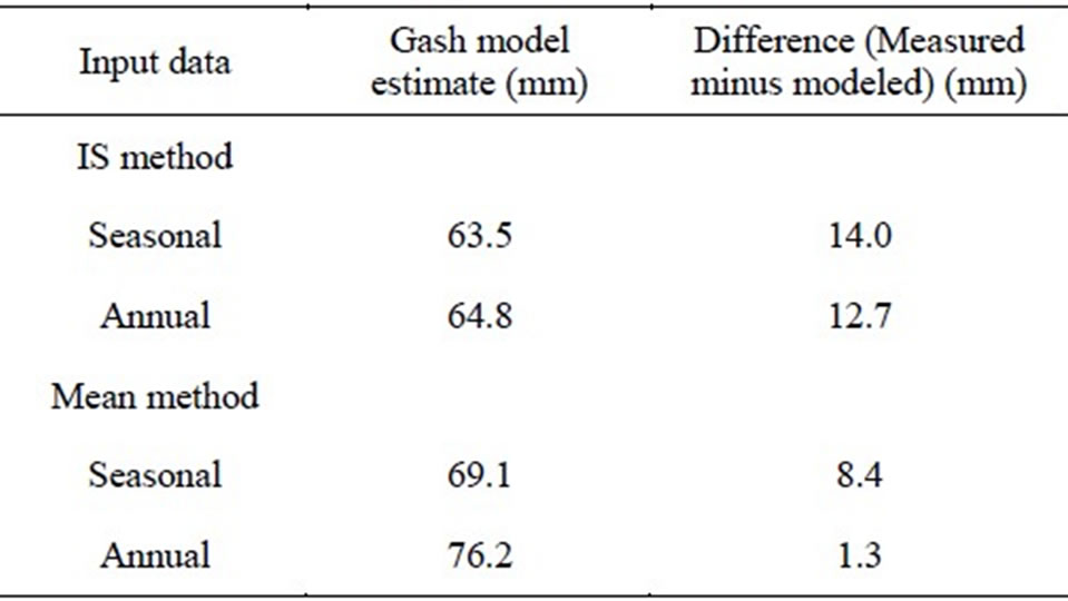
Table 3. Gash model estimates of rainfall interception loss using canopy variables (S, p,  and Ps) derived using the IS method and mean method. Gash model estimates of In were calculated using estimates of the canopy variables for the whole measurement period (annual estimate) or using seasonal estimates of the canopy variables for transition periods (1 May to 20 June and 11 September to 6 November 2007) and for full leaf out periods (25 June to 10 September 2007). The measured interception loss for the storms modeled was 77.5 mm.
would result in estimates of  that are biased toward storms with lower evaporation. The Gash model included the storms with extended rainless periods and subsequently, the IS method underestimated In. In contrast, the mean method used all the storms when estimating S, p,
  and Ps. Hence, for the annual estimates the IS and mean methods estimated
  to be 0.14 and 0.19, respectively. The seasonal estimates for both the IS and mean methods were less accurate and their estimates of
  for both the transition and full leaf out periods were less than 0.19. Regardless of the reason for the differences in Gash model estimates of In, the results demonstrate that the more expensive instrumentation and greater data processing required for the IS method makes it less desirable than the mean method for providing estimates of S, p,
  and Ps for the Gash model. If only an accurate estimate of In is needed, then the mean method is sufficient.
4. Conclusion
The IS method predicted the changes in S and p that are consistent with seasonal changes in the forest canopy for storms with rainfall intensities less than 10 mm·h−1. From May to November, S increased from approximately 0.11 mm in the early spring to 1.2 mm in the summer and then decreased to 0.2 mm after fall senescence. In contrast, p decreased from 0.4 in the early spring to 0.11 in the late summer, only to increase to 0.48 after the leaf abscission. For the study dates, the mean of In was 28%, but ranged between 8% and 100%. When the canopy variables produced by the IS method were applied to the Gash model, the model differed from the measured In by more than 18%. However, the canopy variables provided by the mean method were more accurate and the method is far simpler to use. The IS method is useful for estimating storm to storm variation in S, p,  and Ps, but the estimates of these canopy variables may not as useful for the Gash model when storms have extended rainless periods. Therefore, the IS method holds promise for studies that investigate how canopy parameters affect rainfall interception loss on a per storm basis, but the extra effort and expense required by the IS method is not advantageous for studies that only need an accurate estimate of In. The mean method provided quality estimates for use in the commonly used Gash model.
5. Acknowledgements
We wish to thank the Huron Mountain Wildlife Foundation and the members of the Huron Mountain Club for their generous support. We thank E. Boisvert and N. Karberg for help in the field and W. Thorpe for maintaining the research housing. Funding for this project was provided by the Huron Mountain Wildlife Foundation and USDA McIntire-Stennis.
REFERENCES
- P. J. Zinke, “Forest Interception Studies in the United States,” In: W. E. Sopper and H. W. Lull, Eds., International Symposium on Forest Hydrology, Pergamon Press, New York, 1967, pp. 137-161.
- G. Hörmann, et al., “Calculation and Simulation of Wind Controlled Canopy Interception of a Beech Forest in Northern Germany,” Agricultural and Forest Meteorology, Vol. 79, No. 3, 1996, pp. 131-148. doi:10.1016/0168-1923(95)02275-9
- J. H. C. Gash, “An Analytical Model of Rainfall Interception by Forest,” Quarterly Journal of the Royal Meteorological Society, Vol. 105, No. 443, 1979, pp. 43-55. doi:10.1002/qj.49710544304
- W. Klaassen, “Evaporation from Rain-Wetted Forest in relation to Canopy Wetness, Canopy Cover, and Net Radiation,” Water Resources Research, Vol. 37, No. 12, 2001, pp. 3227-3236. doi:10.1029/2001WR000480
- L. Leyton, E. R. C. Reynolds and F. B. Thompson, “Rainfall interception in forest and moorland,” In: W. E. Sopper and H. W. Lull, Eds., International Symposium on Forest Hydrology, Pergamon Press, New York, 1967, pp. 163-178.
- A. J. Rutter, K. A. Kershaw, P. C. Robins and A. J. Morton, “A Predictive Model of Rainfall Interception in Forests I. Derivation of the Model from Observations in a Plantation of Corsican Pine,” Agricultural Meteorology, Vol. 9, 1971, pp. 367-384. doi:10.1016/0002-1571(71)90034-3
- A. J. Rutte and A. J. Morton, “A Predictive Model of Rainfall Interception in Forests. III. Sensitivity of the Model to Stand Parameters and Meteorological Variables,” Journal of Applied Ecology, Vol. 14, No. 2, 1977, pp. 567-588. doi:10.2307/2402568
- A. J. Rutter, A. J. Morton and P. C. Robins, “A Predictive Model of Rainfall Interception in Forests II. Generalization of the Model and Comparison with Observations in some Coniferous and Hardwood Stands,” Journal of Applied Ecology, Vol. 12, No. 1, 1975, pp. 367-380. doi:10.2307/2401739
- W. Bouten, P. J. F. Swart and E. DeWater, “Microwave Transmission, a New Tool in Forest Hydrological Research,” Journal of Hydrology, Vol. 124, No. 1-2, 1991, pp. 119-130. doi:10.1016/0022-1694(91)90009-7
- W. Klaassen, F. Bosveld and E. de Water, “Water Storage and Evaporation as Constituents of Rainfall Interception,” Journal of Hydrology, Vol. 212-213, 1998, pp. 36-50. doi:10.1016/S0022-1694(98)00200-5
- I. R. Calder and I. R. Wright, “Gamma Ray Attenuation Studies of Interception from Sitka Spruce: Some Evidence for an Additional Transport Mechanism,” Water Resources Research, Vol. 22, No. 3, 1986, pp. 409-417. doi:10.1029/WR022i003p00409
- T. E. Link, M. H. Unsworth and D. Marks, “The Dynamics of Rainfall Interception by a Seasonal Temperate Rainforest,” Agricultural and Forest Meteorology, Vol. 124, No. 3-4, 2004, pp. 171-191. doi:10.1016/j.agrformet.2004.01.010
- M. Herbst, P. T. W. Rosier, D. D. McNeil, R. J. Harding and D. J. Gowing, “Seasonal Variability of Interception Evaporation from the Canopy of a Mixed Deciduous Forest,” Agricultural and Forest Meteorology, Vol. 148, No. 11, 2008, pp. 1655-1667. doi:10.1016/j.agrformet.2008.05.011
- J. H. C. Gash, C. R. Lloyd and G. Lachaud, “Estimating Sparse Forest Rainfall Interception with an Analytical Model,” Journal of Hydrology, Vol. 170, No. 1-4, 1995, pp. 79-86. doi:10.1016/0022-1694(95)02697-N
- NCDC, “Annual Climate Summary,” Marquette, WSO AP, National Climate Data Center, Michigan, 2008.
- J. P. Kimmins, “Some Statistical Aspects of Sampling Throughfall Precipitation in Nutrient Cycling Studies in British Columbian Coastal Forests,” Ecology, Vol. 54, No. 5, 1973, pp. 1008-1019. doi:10.2307/1935567
- L. J. Puckett, “Spatial Variability and Collector Requirements for Sampling Throughfall Volume and Chemistry under a Mixed Hardwood Canopy,” Canadian Journal of Forest Research, Vol. 21, No. 11, 1991, pp. 1581-1588. doi:10.1139/x91-220
- C. R. Lloyd and A. O. Marques Filho, “Spatial Variability of Throughfall and Stemflow Measurements in Amazonian Rainforest,” Agricultural and Forest Meteorology, Vol. 42, No. 1, 1988, pp. 63-72. doi:10.1016/0168-1923(88)90067-6
- H. G. Wilm, “Determining Rainfall under a Conifer Forest,” Journal of Agricultural Research, Vol. 67, No. 12, 1943, pp. 501-512.
- J. B. Stewart, “Modeling Surface Conductance of Pine Forest,” Agricultural and Forest Meteorology, Vol. 43, No. 1, 1988, pp. 19-35. doi:10.1016/0168-1923(88)90003-2
- A. J. Pearce and L. K. Rowe, “Rainfall Interception in a Muli-Storied, Evergreen Mixed Forest: Estimates Using Gash’s Analytical Model,” Journal of Hydrology, Vol. 49, No. 3-4, 1981, pp. 341-353. doi:10.1016/S0022-1694(81)80018-2
- T. E. Link, G. N. Flerchinger, M. H. Unsworth and D. Marks, “Simulation of Water and Energy Fluxes in an Old-Growth Seasonal Temperate Rain Forest Using the Simultaneous Heat and Water (SHAW) Model,” Journal of Hydrometeorology, Vol. 5, No. 3, 2004, pp. 443-457. doi:10.1175/1525-7541(2004)005<0443:SOWAEF>2.0.CO;2
- A. Muzylo, et al., “A Review of Rainfall Interception Modelling,” Journal of Hydrology, Vol. 370, No. 1-4, 2009, pp. 191-206. doi:10.1016/j.jhydrol.2009.02.058
- I. R. Calder, R. L. Hall, P. T. W. Rosier, H. G. Bastable and K. T. Prasanna, “Dependence of Rainfall Interception on Drop Size: 2. Experimental Determination of the Wetting Functions and Two-Layer Stochastic Model Parameters for Five Tropical Tree Species,” Journal of Hydrology, Vol. 185, No. 1-4, 1996, pp. 379-388. doi:10.1016/0022-1694(95)02999-0
- A. G. Price and D. E. Carlyle-Moses, “Measurement and Modelling of Growing-Season Canopy Water Fluxes in a Mature Mixed Deciduous Forest Stand, Southern Ontario, Canada,” Agricultural and Forest Meteorology, Vol. 119, No. 1-2, 2003, pp. 69-85. doi:10.1016/S0168-1923(03)00117-5
- R. F. Keim, “Comment on ‘Measurement and Modeling of Growing-Season Canopy Water Fluxes in a Mature Mixed Deciduous Forest Stand, Southern Ontario, Canada’,” Agricultural and Forest Meteorology, Vol. 124, No. 3-4, 2004, pp. 277-279. doi:10.1016/j.agrformet.2004.02.003
- R. F. Keim and A. E. Skaugset, “A Linear System Model of Dynamic Throughfall Rates Beneath Forest Canopies,” Water Resources Research, Vol. 40, No. 5, 2004, Article ID: W05208. doi:10.1029/2003WR002875
- J. A. Vrugt, S. C. Dekker and W. Bouten, “Identification of Rainfall Interception Model Parameters from Measurements of Throughfall and Forest Canopy Storage,” Water Resources Research, Vol. 39, 2003, p. 1251. doi:10.1029/2003WR002013
- D. E. Carlyle-Moses and A. G. Price, “An Evaluation of the Gash Interception Model in a Northern Hardwood stand,” Journal of Hydrology, Vol. 214, No. 1-4, 1999, pp. 103-110. doi:10.1016/S0022-1694(98)00274-1
- J. D. Helvey and J. H. Patric, “Canopy and Litter Interception of Rainfall by Hardwoods of Eastern United States,” Water Resources Research, Vol. 1, No. 2, 1965, pp. 193-206. doi:10.1029/WR001i002p00193
- L. K. Rowe, “Rainfall Interception by an Evergreen Beech Forest, Nelson, New Zealand,” Journal of Hydrology, Vol. 66, No. 1-4, 1983, pp. 143-158. doi:10.1016/0022-1694(83)90182-8
- R. E. Horton, “Rainfall Interception,” Monthly Weather Review, Vol. 47, No. 9, 1919, pp. 603-623. doi:/10.1175/1520-0493(1919)47<603:RI>2.0.CO;2
- F. André, M. Jonard and Q. Ponette, “Precipitation Water Storage Capacity in a Temperate Mixed Oak-Beech Canopy,” Hydrological Processes, Vol. 22, No. 20, 2008, pp. 4130-4141. doi:10.1002/hyp.7013
- A. M. J. Gerrits, L. Pfister and H. H. G. Savenije, “Spatial and Temporal Variability of Canopy and Forest Floor Interception in a Beech Forest,” Hydrological Processes, Vol. 24, No. 21, 2010, pp. 3011-3025. doi:10.1002/hyp.7712
- G. N. Flerchinger and K. E. Saxton, “Simultaneous Heat and Water Model of a Freezing Snow-Residue-Soil System. I. Theory and Development,” Transactions of the ASAE, Vol. 32, No.2, 1989, pp. 565-571.
- V. G. Jetten, “Interception of Tropical Rainforest: Performance of a Canopy Water Balance Model,” Hydrological Processes, Vol. 10, No. 5, 1996, pp. 671-685. doi:10.1002/(SICI)1099-1085(199605)10:5<671::AID-HYP310>3.0.CO;2-A
- J. H. C. Gash, I. R. Wright and C. R. Lloyd, “Comparative Estimates of Interception Loss from Three Coniferous Forests in Great Britain,” Journal of Hydrology, Vol. 48, No. 1-2, 1980, pp. 89-105. doi:10.1016/0022-1694(80)90068-2
- P. G. Jarvis and D. Fowler, “10: Forests and Atmosphere,” In: J. Evans, Ed., The Forests Handbook, Blackwell Science, Oxford, 2008, pp. 229-281.
- T. Toba and T. Ohta, “An Observational Study of the Factors that Influence Interception Loss in Boreal and Temperate Forests,” Journal of Hydrology, Vol. 313, No. 3-4, 2005, pp. 208-220. doi:10.1016/j.jhydrol.2005.03.003
- Z. Teklehaimanot, P. G. Jarvis and D. C. Ledger, “Rainfall Interception and Boundary Layer Conductance in relation to Tree Spacing,” Journal of Hydrology, Vol. 123, No. 3-4, 1991, pp. 261-278. doi:10.1016/0022-1694(91)90094-X
- A. Deguchi, S. Hattori and H. T. Park, “The Influence of Seasonal Changes in Canopy Structure on Interception Loss: Application of the Revised Gash Model,” Journal of Hydrology, Vol. 318, No. 1-4, 2006, pp. 80-102. doi:10.1016/j.jhydrol.2005.06.005