Open Journal of Forestry
Vol.08 No.01(2018), Article ID:80558,14 pages
10.4236/ojf.2018.81001
Water Use of Juvenile Live Oak (Quercus virginiana) Trees over Five Years in a Humid Climate
Richard C. Beeson1, Hang Thi Thu Duong2, Roger Kjelgren2
1Department of Horticultural Sciences, Institute of Agricultural Sciences, Mid-Florida Research and Education Center, University of Florida, Apopka, FL, USA
2Department of Environmental Horticulture, Institute of Agricultural Sciences, Mid-Florida Research and Education Center, University of Florida, Apopka, FL, USA

Copyright © 2018 by authors and Scientific Research Publishing Inc.
This work is licensed under the Creative Commons Attribution International License (CC BY 4.0).
http://creativecommons.org/licenses/by/4.0/


Received: October 10, 2017; Accepted: November 21, 2017; Published: November 24, 2017
ABSTRACT
To meet minimum spring flows, water management districts in Florida sought to make both agriculture and urban landscapes water efficient, which includes tree farms. Quercus virginiana, commonly known as live oak trees, is endemic to Central Florida and among the most popular landscape trees for their gracefulness and spreading shade. To provide a basis for irrigation allocations both during production and in landscapes, daily actual evapotranspiration (ETA) in liters for three live oak trees was measured with weighing lysimeters over five years, beginning with seedlings and continuing until trees averaged 7.2 meters in height. Empirical models were derived to calculate ETA based on crown horizontal projected area (PCA) or trunk caliper (TCSA), adjusted daily by changes in evapotranspiration (ETO). Average ETA to produce these live oaks was 62,218 L cumulative over 5.5 years. Effectively transpiring leaf, tree water use volume divided by ETO, was closely related to PCA over five years with the slope of this relationship being equivalent to a Plant Factor of 0.93. The product of ETO and this Plant Factor can be used to estimate depth of live oak water demand in urban landscapes. Also, this Plant Factor can estimate water demand volume in nurseries and landscapes when combined with PCA, and similarly the slopes for TCSA can be used to estimate ETA water volume from measured trunk diameter.
Keywords:
Quercus virginiana, Irrigation Scheduling, Irrigation Modelling, Container Production, Landscape Irrigation

1. Introduction
Trees planted in urban landscapes often require irrigation during all stages of life: during production in containers or as large specimens (Beeson, 1992; Beeson & Keller, 2003) , during root system establishment post-transplanting (Gilman, Black, & Dehgan, 1998) , in arid climates (Lindsey & Bassuk, 1991) , or during drought once established in humid climates. Landscape tree water management requires reasonable estimates of water demand in order to schedule irrigation amounts and timing to conserve water while maintaining tree health. Estimating tree water demand is not straightforward. Water demand of isolated trees as typically found in urban landscapes is affected by numerous factors: developmental stages, nutrition, spacing and shading within species, but the overriding are tree size and shape, and transpiration rate (Burger et al., 1987; Fitzpatrick, 1980, 1983; Knox, 1989) .
Defining tree water use terms is critical: we define measured tree evapotranspiration in volume units of liters (L)∙day−1 as whole tree water use (ETA). Further, we define calculated tree transpiration rate in depth units of mm∙day−1 as tree water use rate. Tree water use rate is almost always a derived number calculated from measured ETA divided by some measure of total area of transpiring leaves (Kjelgren, Beeson, Pittenger, & Montague, 2016) . Tree water use rate is typically used in planning or scheduling sprinkler irrigation as water depth, and ETA is used in scheduling irrigation of trees irrigated with drip systems that apply water volume. Finally, we define tree water demand as either volume or depth of tree water use estimated from empirically-derived constants or variables because measuring tree water use rate (mm∙day−1), ETA (L∙day−1) or transpiring leaf (m2) is impractical. Here we have measured ETA with lysimeters and approximated transpiring leaf as the variable, projected crown area (PCA), to derive a Plant Factor, a constant that links the practical use of tree water demand estimation to the most widely accepted variable in managing plant irrigation, reference (or potential) evapotranspiration (ETO; Allen et al., 2005 ). ETO integrates the weather factors of solar radiation, wind, ambient humidity, and air temperature which drive evaporative pull on leaves for a hypothetical clipped cool-season turf, allowing standard measure of potential water demand among places and between times (Allen et al., 2005) .
The literature review of Wullschleger, Meinzer, & Vertessy (1998) reported ETA ranging from 10 to 200 L∙day−1, mostly based on differences in canopy size and transpiring leaf area. Most studies have quantified whole tree evapotranspiration for relatively short periods of time, typically much less than a year or often shorter. Ruiter (1987) studied ETA of Pinus radiata (radiata pine) using large drainage lysimeters with volumes of 7 m3. After three years, trees irrigated throughout the period averaged 3 - 4 m in height, with daily average ETA over four weeks of 21 L∙day−1. Edwards (1986) measured daily ETA of single trees of four species grown in southern New Zealand for a year. At termination, trees ranged from 3.3 to 5.6 m in height. ETA exceeded 120 L∙day−1 in summer for Ecualyputus fastigata, and was near zero for deciduous species during winter. Beeson (2016) quantified average ETA of three Acer rubrum trees using weighing lysimeters (Beeson, 2011) from small liners to 8 m tall trees over five years in Central Florida. Total average volume of three trees was 29,107 L cumulative over nearly five years. During the summer months of the last year, ETA peaked at 101 L∙day−1.
In an experiment of five species of containerized woody plants, Knox (1989) described the primary factors driving whole tree water use as transpiration rates and size. In Central Florida Beeson (1993) compared water use rate (mm∙day−1) of container grown (10.2 L) Rhododendron sp. “Formosa” to water demand estimated from the ETO (Penman-Monteith equation, cool season turfgrass reference) corrected by a Plant Factor. The study noted that poor correlations between estimated demand and measured water use rate can be improved by more frequent canopy measurements to capture size changes during periods of rapid growth. Devitt, Morris, & Neuman (1994) , measured ETA of three woody ornamentals in order to improve water demand estimates of Prosopis alba Grisebach, Chilopsis linearis (Cav.) Sweet var. linearis and Quercus virginiana Mill. in Nevada. They found ETA of oak was closely correlated to all measured growth parameters, defined as height, diameter, and canopy volume.
St.Clair (1994) suggested that water use be estimated from trunk diameter. Although ETA was related to trunk diameter, the relationship was nonlinear. Simpson (2000) reported that ETA in L∙day−1 was related to the cross-sectional sapwood area, a more finely-tuned measure of xylem water conducting capacity than trunk diameter. However sapwood area depends on tree species and tree age. For Acer rubrum, a diffuse-porous species, correlation between ETA and trunk cross sectional area was shown to be valid for trees up to 100 years of age (Gebauer, Horna, & Leuschner, 2008) . But for a ring porous species, such as Quercus sp., this relationship may only be valid for young trees (Greenridge, 1955; Kozlowski & Winget, 1963) . Quercus sp. are ring porous, so may have a lower correlation between ETA and trunk cross sectional area in mature trees (Kramer & Kozlowski, 1979) . Stem cross-sectional area can still be an easily measured estimate of leaf area, and so useful in estimating whole plant water use. Weighing lysimeters are the most precise tool for empirically measuring whole plant water use, and so the basis for developing Plant Factors that combine with ETO to estimate tree water demand in nurseries and landscapes.
Most tree water use studies have been conducted in semi-arid to arid climates; much less so in humid climates. More information on estimating tree water demand in humid climates, either as a rate or as a volume, can aid nursery and landscape water managers and policy makers in humid regions, especially in subtropical climates with lengthy dry seasons. Our objective was to use tree water use volumes (ETA) measured from lysimeters to model evapotranspiration rates with measures of tree size such as projected canopy area and trunk cross sectional areas of live oak, a common landscape tree in warm temperate and sub-tropical climates. Findings presented here are daily mean ETA and growth of three individual oak trees beginning from seedlings to 7.2 m tall trees over nearly six years. The objective of this study was to develop Plant Factors from measured ETA (volume unit) and ETO. Here we used easily measured tree traits that control transpiration, projected canopy area and trunk cross sectional area, such that whole tree water demand can be estimated for improved water management in nursery production and irrigated landscapes.
2. Materials and Methods
2.1. Experimental Setup
2.1.1. Transplanting
Live oak seedlings (Quercus virginiana) were obtained late winter 2001from a nursery in north Central Florida. Seedlings were relocated 75 Km east of the nursery to within the Orlando, Florida Metropolitan area (28.54 latitude and −81.38 longitude). Five seedlings were transplanted into 26 L containers using a 70% composted pine bark: 30% Florida sedge peat: 10% coarse sand substrate amended with 0.68 kg∙per∙m3 of micronutrients Micromax (Scotts Company, Marysville, OH) and 2.3 kg∙per∙m3 of dolomite limestone to buffer to a pH of 6.0. In years 2004-2005, NuPeat, composed from one-third composted yard waste, one-third composted and screened hardwood bark, and one-third Florida sedge peat, replaced existing sedge peat. These five containers were painted inside with a latex paint mixed with copper (Spin-out, Griffin Corp, Vadosta, GA) and the outside covered with aluminum foil to reduce excess container heating and surface evaporation. These containers were also covered with a shallow convex dome to exclude most rainfall and to reduce evaporation from the container substrate. Each subsequent study year, trees were planted during late winter into sequentially larger containers, with the same substrate, fertilization, and container prep followed. In 2002, trees were transplanted in 95 L container (0.55 m diameter), then in each subsequent year 2002-2005 trees were progressively moved into 361,760, and 1140 L containers. In 2003 an appropriately-sized wire basket (32-COT, Cherokee Manufacturing Inc., St. Paul, MN) was placed in containers to maintain root ball integrity while lifting trees during replanting into larger containers without causing damage to trunks.
2.1.2. Tree Care
Trees were staked, pruned, and fertilized as needed using controlled release fertilizer (Polygon 19N-4.2P-11.6K, Harrell’s Fertilizer Co. Lakeland, FL). Starting in 2002, overall tree canopies were pruned to promote tree structure in accordance with Florida Grades and Standards for Nursery Crops mid-to-late winter (Florida Department of Agriculture and Consumer Services, 1998) . In 2003, after transplanting, trees were pruned to raise the bottom of tree canopies to 1.2 m above the root ball.
2.2. Experimental Layout
The first year, five study trees were suspended from a 2 m high tripod lysimeter (Beeson, 2011) which consisted of a basket to hold the container suspended from a load cell (SSM-100, Interface Force Inc., Scottsdale, AZ) underneath the tripod. Load cells were connected to a data logger (CR10X, Campbell Scientific, Inc., Logan, UT) and multiplexer system (AM-416 and AM-32) that collected lysimeter mass every half hour and controlled irrigation (Beeson, 2011) . In 2002, the three largest trees were placed singly in large weighting lysimeters (Beeson, 2011) in a row oriented east-west. Each triangular lysimeter basket was suspended from three 341 kg load cells (SSM-750, Interface Force Inc., Scottsdale, AZ) attached to steel pillars at apices. A basket accommodated up to a 1.55 m diameter polyethylene container. Study trees remained in the triangular lysimeters from 2002 through 2006.
Spacing of border trees each spring was representative of nursery production at each stage of growth. In 2001 trees were 0.4 m on center using a square arrangement with 95 border trees handled and transplanted the same as the study trees. Lysimeters were randomly placed within a middle row in the block of four rows of 25 containers. In 2002, 18 border trees were transplanted into containers similar to those of the study trees and placed around each triangular lysimeter study tree to maintain tree canopy cover, which provided an initial canopy density of 50%, approximating that of a commercial nursery. In 2003, border trees were reduced to 12 per lysimeter to maintain 50% canopy density. In 2004, the number of border trees around each lysimeter was reduced to six to maintain constant canopy density. In 2005, one border tree was placed in the four cardinal directions around each lysimeter, with one tree between lysimeters within the row.
2.3. Irrigation
The first year, five study trees were suspended from a 2 m high tripod lysimeter (Beeson, 2011) which consisted of a basket to hold the container suspended from a load cell (SSM-100, Interface Force Inc., Scottsdale, AZ) underneath the tripod. Load cells were connected to a data logger (CR10X, Campbell Scientific, Inc., Logan, UT) and multiplexer system (AM-416 and AM-32) that collected lysimeter mass every half hour and controlled irrigation (Beeson, 2011) . In 2002, the three largest trees were placed singly in large weighting lysimeters (Beeson, 2011) in a row oriented east-west. Each triangular lysimeter basket was suspended from three 341 kg load cells (SSM-750, Interface Force Inc., Scottsdale, AZ) attached to steel pillars at apices. A basket accommodated up to a 1.55 m diameter polyethylene container. Study trees remained in the triangular lysimeters from 2002 through 2006.
Spacing of border trees each spring was representative of nursery production at each stage of growth. In 2001 trees were 0.4 m on center using a square arrangement with 95 border trees handled and transplanted the same as the study trees. Lysimeters were randomly placed within a middle row in the block of four rows of 25 containers. In 2002, 18 border trees were transplanted into containers similar to those of the study trees and placed around each triangular lysimeter study tree to maintain tree canopy cover, which provided an initial canopy density of 50%, approximating that of a commercial nursery. In 2003, border trees were reduced to 12 per lysimeter to maintain 50% canopy density. In 2004, the number of border trees around each lysimeter was reduced to six to maintain constant canopy density. In 2005, one border tree was placed in the four cardinal directions around each lysimeter, with one tree between lysimeters within the row.
2.4. Climate Conditions
Climatic conditions in Central Florida during the 5 year the experiment were conducted as considered normal. During January to mid-March, temperatures normally ranged from 4˚C to 20˚C most days with mostly sunny conditions. Temperatures below freezing were infrequent, but occurred. From late March late May, sunny skies continued, with infrequent rain storms and rapidly increase in temperatures. In late May, temperatures ranged from 24˚C to 32˚C with frequent thunderstorms that continued to mid-October. From mid-October to late November, temperature ranges were similar to spring, with night temperatures dropping below 5˚C and occasional freezes. During this 5 year period, several hurricanes impacted the research site with some leaf loss.
2.5. Data Collection
2.5.1. Reference Evapotranspiration
Reference evapotranspiration (ETO) was calculated each day from a Campbell Scientific (Logan, UT) weather station located in a grassy field 25 m west of lysimeters. The weather station consisted of a pyranometer (Li-200; Li-Cor Inc., Lincoln, NE), a tipping bucket rain gauge (TE525, Texas, Instruments, Dallas, TX), temperature/humidity sensor (CS-215, Campbell Scientific Inc., Logan, UT), a wind sensor (Model 014, Met One Instruments, Grants Pass, OR), and a CR10X data logger that used Application Note 4 (Campbell Scientific Inc.) to calculate ETO with resistance as described by Allen, Jensen, Wright, & Burman (1989) .
2.5.2. Growth Measurements
Growth measurements of tree height, branch spread of widest width and width perpendicular, and maximum trunk caliper at 0.15 m and 0.30 m above the substrate were recorded on lysimeter trees every three weeks during each growing season for the first three years. Beginning year three, trunk circumference was measured with a metal tape measure. At the beginning of the last third of year two, trunk circumference measurements were initiated at 1.2 m above the substrate. Horizontal Projected Canopy Area (PCA, m2) was calculated by multiplying consistent perpendicular measurements of branch spread, north-south and east-west. Trunk cross sectional area (TSCA, cm2) was calculated for each of three trunk measurement based on trunk circumference; where circumference divided by 6.284 (=2*π) equals trunk diameter. Diameter divided by 2, then multiplied by 9.689 (π2) equalizes cross sectional area was calculated as: Area = radius2 × π. (http://www.sengpielaudio.com/calculator-cross-section.htm).
2.5.3. Water Use
Usually ETA was calculated daily as differences between mass recorded at 6:00 am minus mass recorded at 10:00 pm. When partial midday irrigation was in effect, increases in mass from midday irrigation was calculated by the datalogger and added to the daily sum. However, if rare loss of power or common rain events occurred between 6:00 am and 10:00 pm, actual daily cumulative ETA was estimated as described by Beeson (2006) . For power loss, each tree’s daily ETA before and after the loss was normalized to water volume per unit ETO (Normalized ETO, L∙mm−1). This assumed leaf area was constant and normalized values varied minimally over short periods of four to seven days without precipitation. Daily ETA for each missing day was estimated by multiplying the Normalized ETO volume by the measured ETO for each missing day. When rainfall occurred between 6:00 am and 10:00 pm, half hour mass data was plotted to indicate rainfall events. Periods of decreases in mass were summed to estimate ETA. This was then vetted by normalizing by ETO, then comparing the rain day normalized ETA to normalized ETA of recent rainless days.
2.6. Data Analysis
Daily volumetric water use and average daily air temperature were plotted over the growing season for each year. Measurements of tree cross sectional areas that control transpiration (PCA and TSCA at three heights, in m2) were regressed against corresponding Normalized ETA (N-ETA; ETA ÷ ETO in liters mm−1) on days trees were measured. PCA and TSCAs were averaged each quarter each year and plotted over growing season throughout 5.75 years. Pooled standard deviation for three trees was calculated for each quarter. Linear regression was analyzed in R 3.4.1 using simple linear regression model.
3. Results
3.1. Quantifying ETA
Live oak is a medium-fast growth evergreen tree under well-irrigated conditions. Trees grew from 0.22 m to 7.18 m tall over 5.75 years with an average increase of 1.30 m/year in height for the first 3.75 years, and a slower increased height of 1.0 m/year for the last 1.75 years. Leaf habit is evergreen, with leaves slowly shedding, buds bursting and leaves expanding on spur shoots for several weeks in February to early March, with first major shoot elongation occurring usually in mid-April, thus leaf area was relatively constant or increasing throughout the experiment. Bell-shaped variations in ETA over a year are therefore reflective of three distinct shoot flushes and changes in weather―temperature, sun, humidity, and day length―which drove ETO, along with changes in leaf accumulation. These bell shapes had longer tails during winter and early spring due to lower temperatures, solar radiation, and leaf change, covering the approximate first third of each year. As shown in Figure 1(a), the height of the bell shapes increased over years due to the leaf area increases throughout the experiment. In an area with high humidity such as Florida, seasonal changes in ETA reflect temperature changes rather than that of solar radiation. Figure 1(b) shows changes in daily average temperature throughout the experiment.
Year 1, trees grew from 0.22 m to 1.58 m tall, and from 0.11 m to 0.57 m in average canopy spread by the end of December. ETA gradually increased from mid-April (around day 100), peaked at the end of July and mid-October, and then gradually declined from mid-October onward. Mean cumulative ETA from April to December for 2001 was 123.7 L with daily ETA as 0.46 L∙day−1 (data not shown). Year 2, trees initiated bud break in mid-February, concurrent with slow defoliation of the previous leaves, followed by a large leaf flush from early May to mid-August. There was another full leaf flush from mid-September to early October. Tree height increased from 1.59 to 2.94 m and average canopy spread increased from 0.57 m to 1.83 m. Mean cumulative ETA for the entire year was 1395.6 L, with daily ETA greatly increased to 3.8 L∙day−1, as shown in Figure 1(a). Year 3, initial bud break occurred again in early February, with first spur leaf flush occurring as in previous years, in mid-February; the second full leaf flush occurred from early to late May. ETA in the third year was approximately three-fold larger than that of the second year, increasing to 13.52 L∙day−1, with a mean cumulative ETA of 4933.75 L. Trees grew from 2.94 m to 4.26 m tall and from 1.54 m to 2.81 m in average canopy spread. Year 4, bud break began in early February with three full leaf flushes from mid to late March, early to mid-May and early July to early August. Trees grew from 4.31 m to 5.46 m tall and from 2.81 m to 3.73 m in average canopy spread. Daily ETA doubled to 3,166 L∙day−1 compared to the previous year. Figure 1(a) shows mean cumulative ETA for the fourth year was 11,586.7 L. Bud break and duration varied slightly from year-to-year. Year 5, transition bud break began in March, with the first full leaf flush lasting a month starting in early April and the second full leaf flush occurred in early June to late June, extending to late July. Trees averaged from 5.90 m to 6.54 m in height and from 3.81 m to 4.62 m in average canopy spread by the end of December. As shown in Figure 1(a), daily ETA for the fifth year again more than double that of the fourth year to 59.21 L∙day−1 with a mean cumulative ETA of 21,612.84 L. In the last year, until August when the trees were harvested, the height reached 7.18 m and average canopy spread to 4.85 m, with cumulative ETA of 22,565.49 L, and daily ETA of 93.63 L∙day−1.
3.2. Modelling Daily ETA
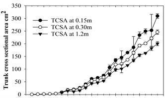
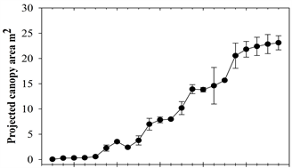
Projected Canopy Area (PCA) and Trunk Cross Sectional Areas (TCSA) were calculated at 0.15 m, 0.3 m, and 1.2 m and, as shown in Figure 2, steadily increased over time. PCA slightly decreased or was level in the first quarter each year because trees were pruned during late February to early March, depending on the year. Thereafter growth quickly recovered.

Figure 1. Mean daily ETA of Quercus virginiana (live oak) and mean daily temperature in Apopka, Florida from 2001 to 2006. Note. (a) Each point is based on the mean of three trees replicates; (b) Data obtained from FAWN: Florida Automatic Weather Network.
 (a)
(a)
 (b)
(b)
Figure 2. Average quarterly projected canopy area (a) and trunk cross sectional (b) for Quercus viriginia. Note: for both (a) and (b) each point is the average of three tree replicates; (b) measured 0.15 m, 0.30 m, and 1.2 m at the first major branch above the soil.
N-ETA was closely and linearly related to the four measures of tree size (r2 ≥ 0.85 and Pr(>F) = 2.26e−16 for all four relationships; Figure 2). Algebraically rearranging the fitted Equation (1) to solve for ETA yields:
 (1)
(1)
The relationship between N-ETA and TCSA at all trunk heights was slightly closer and more linear over years than with the measures of PCA at 1.2 m, as shown in Figure 3. Slopes for each equation can be used as coefficients to estimate ETA (in liters) which can be redefined as water demand for a given duration based on what time period ETO represents, either the previous day or a cumulative number of days.
3.3. Discussion
Tree growth resulted in about 1.0 m to 1.3 m of height growth each year. Long growing seasons in Central Florida likely compensated for shorter days (14 hr
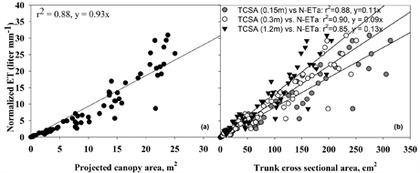
Figure 3. Relationships of normalized ETA over 6 years to four measures of horizontal surface areas. Horizontal projected canopy area, (b) Trunk cross sectional areas at 0.15 m, 0.30 m, and 1.2 m (first major branch) above the soil of Quercus viriginia to estimate daily ETA. The P value Pr(>F) = 2.26e−16, was the same for all four relationships.
maximum) and warmer nights compared to northern latitudes. ETA of the live oak trees was maintained quite low for 2 - 3 months of winter due to relatively low temperatures (20˚C to 25˚C daily Tmax; 10˚C to 15˚C Tmin) and low solar radiation which resulted in slow growth of trees. ETA gradually increased in spring with bud break with warmer temperatures (25˚C to 30˚C daily Tmax; 20˚C to 23˚C Tmin) and longer days, increasing ETO from average 2.6 mm∙day−1 in winter to 5.05 mm∙day−1 in spring, as shown in Figure 1. The bell-shaped pattern of ETO tightly reflects seasonal variability in temperature of the northern hemisphere. The result is in contrast with deciduous maple tree reported by Beeson (2016) that daily ETA rapidly declined due to shoot growth termination even though ETO remained fairly consistent into September.
Water use of Quercus sp. reveals important relationships to environmental conditions that have not been previously reported. Compared to other previously reported landscape trees, ETA values of live oak trees were similar in the first five years at the height of 6.5 m, but much higher in the sixth year (93.63 L∙day−1) at the height of 7.2 meters. Pausch, Grote, & Dawson (2000) reported daily ETA rates of 61 to 72 L∙day−1 for Acer saccharum in forest near Ithaca, NY for 24 cm DBH trees. Under similar conditions and experimental setup, red maple trees (Acer rubrum L.) in Florida average ETA was 29,107 L cumulative over nearly five years for trees 0.4 m to 8 m tall (Beeson, 2016) , and cumulative holly (Ilex spp.) ETA was 20.461 L per tree over nearly six years from 0.3 m to 4.3 m tall (Beeson, Duong, & Kjelgren, 2017) . Whereas cumulative ETA of live oak over nearly six years was 3-fold higher than that of holly at 62,218 L for trees 0.22 m to 7.18 m tall.
Given the data here, and that leaf area and sapwood area are generally closely related, sapwood area can serve as a predictor of volumetric water demand for individual trees, even for a ring porous species such as live oak, either directly as a variable when combined ETO and an appropriate Plant Factor (see Equation (1)), or used to estimate PCA, which could then be used in Equation (1). In a study of water use of Interior West Douglas-fir (Pseudotsuga menzezii var. glauca) in a natural environment, Simpson (2000) found that for small trees a large portion of basal area (total cross-sectional area of stem at 1.5 m) was sapwood area. Similarly, Sellin (1991) found for a 10-year old dominant Norway spruce (Picea abies (L.) Karst.) that approximately 95% of the stem cross-sectional area was conducting sapwood and so contributing to whole plant water use. PCA or TCSA, therefore, can be a relatively good indicator of maximum whole plant potential water use for individual trees when combined with ETO and a Plant Factor appropriate to PCA or TCSA.
A key point of this study is that the slope of the relationship between N-A, which is an estimate of transpiring leaf area after variability from ETO is factored out, and PCA is equivalent to the Plant Factor described by Kjelgren et al. (2016) . Past tree water use studies often divided ETA by laboriously harvested total leaf area that may not be the best measure of transpiring leaf area. Harvested total leaf area will include many leaves that are shaded over the course of a day, especially species with dense crowns, so would contribute little to ETA. PCA is perhaps a less precise measure than TCSA but is probably a simpler and practical means to estimate transpiring leaf area, and with a proper Plant Factor, a more useful way to estimate volumetric tree water demand.
Correlation between N-ETA with PCA and TCSA at heights of 0.15 m, 0.30 m, and 1.2 m of the oak trees was high, r2 ≥ 0.85 Pr(>F) = 2.26e−16, was the same for all four relationships, and similar to the relationships between ETA and the same growth parameters that were found for red maple (Beeson, 2016) and holly (Beeson et al., 2017) . Trunk diameter is closely correlated with tree size and leaf area (Martin, Kloeppel, Schafer, Kimbler, & McNulty, 1998; Simpson, 2000; Vertessy, Benyon, O’Sullivan, & Gribben, 1995) of diffuse-porous species because conducting xylem area is continuous and proportional to transpiring leaf area, and so leaf area correlates with water use under a given set of environmental conditions (Beeson, 1997; McDermitt, 1990; Teskey & Sheriff, 1996; Vertessy et al., 1995) . For individual species, leaf area and cross-sectional sapwood area are closely related to ETA in balsam fir (Abies balsamea (L.) Mill.) (Coyea & Margolis, 1992) , mountain ash (Eucalyptus regnans F.J. Muell.), silver wattle (Acacia dealbata Link.) (Vertessy et al., 1995) and Monterey pine (Pinus radiata D. Don) (Teskey & Sheriff, 1996) .
4. Conclusion
Daily ETA of Quercus virginiana can be estimated with high precision based on current methods of calculating ETO and using the appropriate coefficients (for PCA or TCSA) for a given measure of tree capacity to move and transpire water, as shown in Figure 3. The three measures using TCSA to estimate water demand (ETA) are suited to nursery production where trunk diameter (caliper) is a routine measure for marketing classification, but can be used for isolated landscape trees with due consideration. Extrapolations beyond live oak tree sizes measured here are possible and would be most accurate if based on trunk cross sectional area closely below the bottom of first branch, where the greatest reduction of water conducting vessels occurs before transpiration by leaves. However, for larger live oak with more non-conducting heartwood, the relationships between N-ETA and TCSA would be much more uncertain. Projected canopy area is a more useful approach to estimated whole tree-volumetric water demand not affected by uncertainties in conducting sapwood area in older specimens or ring porous species. The coefficient (slope) for either PCA or TSCA that corrects calculated ETO to live oak water use is dimensionless, but to estimate in volume units (either liters or gallons) would require both ETO and PCA/TCSA to be in the same class of units, metric or English.
Acknowledgements
Funding for this project was provided by the Southwest Florida Water Management District and the Horticulture Research Institute.
Cite this paper
Beeson, R. C., Duong, H. T. T., & Kjelgren, R. (2018). Water Use of Juvenile Live Oak (Quercus virginiana) Trees over Five Years in a Humid Climate. Open Journal of Forestry, 8, 1-14. https://doi.org/10.4236/ojf.2018.81001
References
- 1. Allen, R. G., Jensen, M. E., Wright, J. L., & Burman, R. D. (1989). Operational Estimates of Reference Evapotranspiration. Journal of Agronomy, 81, 650-662.https://doi.org/10.2134/agronj1989.00021962008100040019x [Paper reference 1]
- 2. Allen, R. G., Walter, I. A., Elliot, R., Howell, T., Itenfisu, D., & Jensen, M. (2005). The ASCE Standardized Reference Evapotranspiration Equation. Moscow, ID: University of Idaho, Kimberly Research and Extension Center, Environmental and Water Resources Institute of the American Society of Civil Engineers https://www.kimberly.uidaho.edu/water/asceewri/ascestzdetmain2005.pdf [Paper reference 2]
- 3. Beeson Jr., R. C. (1992). Restricting Overhead Irrigation to Dawn Limits Growth in Container-Grown Woody Ornamentals through Small Increases in Diurnal Water Stress. HortScience, 27, 996-999. [Paper reference 1]
- 4. Beeson Jr., R. C. (1993). Relationship of Potential Evapotranspiration and Actual Evapotranspiration of Rhododendron sp. ‘Formosa’. Proceedings of the Florida State Horticultural Society, 106, 274-276. http://fshs.org/proceedings-o/1993-vol-106/274-276%20(BEESON).pdf [Paper reference 1]
- 5. Beeson Jr., R. C. (1997). Using Canopy Dimensions and Potential Evapotranspiration to Schedule Irrigation of Ligustrum japonicum. Proceedings of the Southern Nursery Association Research Conference, 42, 413-416. [Paper reference 1]
- 6. Beeson Jr., R. C. (2006). Relationship of Plant Growth and Actual Evapotranspiration to Irrigation Frequency Based on Managed Allowable Deficits for Container Nursery Stock. Journal of the American Society of Horticultural Science, 131, 140-148. [Paper reference 1]
- 7. Beeson Jr., R. C. (2011). Weighing Lysimeter Systems for Quantifying Water Use and Studies of Controlled Water Stress for Crops Grown in Low Bulk Density Substrates. Agricultural Water Management, 98, 967-976. https://doi.org/10.1016/j.agwat.2011.01.005 [Paper reference 7]
- 8. Beeson Jr., R. C. (2016). Evapotranspiration and above Ground Biomass of Acer rubrum from Liners to 8m Tall Trees. American Journal of Plant Sciences, 7, 2440-2456.https://doi.org/10.4236/ajps.2016.717213 [Paper reference 4]
- 9. Beeson Jr., R. C., & Keller, K. (2003). Effect of Cyclic Irrigation on Growth of Magnolias Produced Using Five In-Ground Systems. Journal of Environmental Horticulture, 21, 148-152. [Paper reference 1]
- 10. Beeson Jr., R. C., Duong, H. T. T., & Kjelgren, R. J. (2017). Developing a Simple Water Use Model for Ilex x ‘Nellie R Stevens’ from Liners to Four Meter Tall Trees. Journal of Agricultural Studies, 5, 83-96. [Paper reference 2]
- 11. Burger, D. W., Hartin, J. S., Hodel, D. R., Lukaszewski, T. A., Tjosvold, S. A., & Wagner, S. A. (1987). Water Use in California’s Ornamental Nurseries. California Agriculture, 41, 97-104. [Paper reference 1]
- 12. Coyea, M. R. & Margolis, H. A. (1992). Factors Affecting the Relationship between Sapwood Area and Leaf Area of Balsam Fir. Canadian Journal of Forest Research, 22, 1684-1693. https://doi.org/10.1139/x92-222 [Paper reference 1]
- 13. Devitt, D. A., Morris, R. L., & Neuman, D. S. (1994). Evapotranspiration and Growth Response of Three Woody Ornamental Species Placed under Varying Irrigation Regimes. Journal of the American Society for Horticultural Science, 119, 452-457. [Paper reference 1]
- 14. Edwards, W. R. N. (1986). Precision Weighing Lysimetry for Trees, Using a Simplified Tared-Balance Design. Tree Physiology, 1, 127-144. https://doi.org/10.1093/treephys/1.2.127 [Paper reference 1]
- 15. Fitzpatrick, G. (1980). Water Budget Determinations for Container-Grown Ornamental Plants. Proceedings of the Florida State Horticultural Society, 93, 166-168.http://fshs.org/proceedings-o/1980-vol-93/166-168%20(FITZPATRICK).pdf [Paper reference 1]
- 16. Fitzpatrick, G. (1983). Relative Water Demand in Container-Grown Ornamental Plants. HortScience, 18, 760-762. [Paper reference 1]
- 17. Florida Department of Agriculture and Consumer Services (1998). Grades and Standards for Nursery Plants (2nd ed.). Tallahassee: Author. [Paper reference 1]
- 18. Gebauer, T., Horna, V., & Leuschner, C. (2008). Variability in Radial Sap Flux Density Patterns and Sapwood Area among Seven Co-Occurring Temperate Broad-Leaved Tree Species. Tree Physiology, 28, 1821-1830. https://doi.org/10.1093/treephys/28.12.1821 [Paper reference 1]
- 19. Gilman, E. F., Black, R. J., & Dehgan, B. (1998). Irrigation Volume and Frequency and Tree Size Affect Establishment Rate. Journal of Arboriculture, 24, 1-9. [Paper reference 1]
- 20. Greenridge, K. N. H. (1955). Observations on the Movement of Moisture in Large Woody Stems. Canadian Journal of Botany, 33, 202-221. https://doi.org/10.1139/b55-016 [Paper reference 1]
- 21. Kjelgren, R., Beeson, R. C., Pittenger, D. R., & Montague, D. T. (2016). Simplified Landscape Irrigation Demand Estimation: SLIDE Rules. Applied Engineering in Agriculture, 32, 363-378. https://doi.org/10.13031/aea.32.11307 [Paper reference 2]
- 22. Knox, G. W. (1989). Water Use and Average Growth Index of Five Species of Container Grown Woody Landscape Plants. Journal of Environmental Horticulture, 7, 136-139. [Paper reference 2]
- 23. Kozlowski, T. T., & Winget, C. H. (1963). Patterns of Water Movement in Forest Trees. Botanical Gazette, 124, 301-311. http://www.jstor.org/stable/2472915 https://doi.org/10.1086/336210 [Paper reference 1]
- 24. Kramer, P. J., & Kozlowski, T. T. (1979). Physiology of Woody Plants. New York, NY: Academic Press, Inc. [Paper reference 1]
- 25. Lindsey, P., & Bassuk, N. (1991). Specifying Soil Volumes to Meet the Water Needs of Mature Urban Street Trees and Trees in Containers. Journal of Arboriculture, 17, 141-149. [Paper reference 1]
- 26. Martin, J. G., Kloeppel, B. D., Schaefer, T. L., Kimbler, D. L., & McNulty, S. G. (1998). Aboveground Biomass and Nitrogen Allocation of Ten Deciduous Southern Appalachian Tree Species. Canadian Journal of Forest Research, 28, 1648-1659. https://doi.org/10.1139/x98-146 [Paper reference 1]
- 27. McDermitt, D. K. (1990). Sources of Error in the Estimation of Stomatal Conductance and Transpiration from Porometer Data. HortScience, 25, 1538-1548. [Paper reference 1]
- 28. Pausch, R. C., Grote, E. E., & Dawson, T. E. (2000). Estimating Water Use by Sugar Maple Trees: Considerations When using Heat-Pulse Methods in Trees with Deep Functional Sapwood. Tree Physiology, 20, 217-227. https://doi.org/10.1093/treephys/20.4.217 [Paper reference 1]
- 29. Ruiter, J. H. (1987). Growth, Crop Conductance and Prediction of Stem Volume Increment of Irrigated and Non-Irrigated Young Radiata Pine in Non-Weighing Lysimeters. Forest Ecology and Management, 20, 79-96. https://doi.org/10.1016/0378-1127(87)90151-4 [Paper reference 1]
- 30. Sellin, A. (1991). Variation in Sapwood Thickness of Picea abies in Estonia Depending on Tree Age. Scandinavian Journal of Forest Research, 6, 463-469. https://doi.org/10.1080/02827589109382683 [Paper reference 1]
- 31. Simpson, D. G. (2000). Water Use of Interior Douglas-Fir. Canadian Journal of Forestry Research, 30, 534-547. https://doi.org/10.1139/x99-233 [Paper reference 3]
- 32. St.Clair, J. B. (1994). Genetic Variation in Tree Structure and Its Relation to Size in Douglasfir. I. Biomass Partitioning, Foliage Efficiency, Stem Form, and Wood Density. Canadian Journal of Forestry Research, 24, 1226-1235. https://doi.org/10.1139/x94-161 [Paper reference 1]
- 33. Teskey, R. O., & Sheriff, D. W. (1996). Water Use by Pinus radiata Trees in a Plantation. Tree Physiology, 16, 273-279. https://doi.org/10.1093/treephys/16.1-2.273 [Paper reference 2]
- 34. Vertessy, R. A., Benyon, R. G., O’Sullivan, S. K., & Gribben, P. R. (1995). Relationships between Stem Diameter, Sapwood Area, Leaf Area and Transpiration in a Young Mountain Ash Forest. Tree Physiology, 15, 559-567. https://doi.org/10.1093/treephys/15.9.559 [Paper reference 3]
- 35. Wullschleger, S. D., Meinzer, F. C., & Vertessy, R. A. (1998). A Review of Whole-Plant Water Use Studies in Trees. Tree Physiology, 18, 499-512. https://doi.org/10.1093/treephys/18.8-9.499 [Paper reference 1]