Open Journal of Acoustics
Vol.3 No.2A(2013), Article ID:33050,7 pages DOI:10.4236/oja.2013.32A001
Power Estimation of Acoustic Sources by Sensor Array Processing
Department of Applied Mechanics, Institute Franche-Comté Electronique Mécanique Thermique et Optique-Sciences et Technologies, University of Franche-Comté, Besançon, France
Email: joseph.lardies@univ-fcomte.fr
Copyright © 2013 Joseph Lardiès et al. This is an open access article distributed under the Creative Commons Attribution License, which permits unrestricted use, distribution, and reproduction in any medium, provided the original work is properly cited.
Received April 9, 2013; revised May 9, 2013; accepted May 16, 2013
Keywords: Array Signal Processing; Acoustic Array; Acoustic Power Estimation; Beamforming; Far Field
ABSTRACT
A constant problem is to localize a number of acoustic sources, to separate their individual signals and to estimate their strengths in a propagation medium. An acoustic receiving array with signal processing algorithms is then used. The most widely used algorithm is the conventional beamforming algorithm but it has a very low resolution and high sidelobes that may cause a signal leakage problem. Several new signal processors for arrays of sensors are derived to evaluate the strengths of acoustic signals arriving at an array of sensors. In particular, we present the covariance vector estimator and the pseudoinverse of the array manifold matrix estimator. The covariance vector estimator uses only the correlations between sensors and the pseudoinverse of the array manifold matrix estimator operates with the minimum eigenvalues of the covariance matrix. Numerical and experimental results are presented.
1. Introduction
Arrays of sensors are used in many fields to detect weak signals, to estimate the bearing and the strengths of signals arriving from different directions. For example, in industrial environment an array of microphones is used to localize and to determine the strength of polluting noise sources. Conventional ways of noise source identifications include sound intensity measurement [1] and acoustic holography [2] but these techniques suffer from the drawbacks of being restricted in only small areas or short distances and cannot be applied in far fields or in a complex industrial environment. In this study, we propose array processing algorithms which are useful in identifying acoustic sources in the far field of the array. Excellent text regarding the fundamental aspects of array signal processing techniques can be found in Stoica et al. [3]. Shan et al. proposed in [4] a spatial smoothing technique to resolve the multipath problem in narrowband beamforming. Schmidt developed in [5] a multiple signal classification (MUSIC) algorithm that is essentially an eigenvalues-based approach to significantly improve the resolution of multiple sources. The extension of MUSIC in the presence of steering vector errors was developed in [6]. Yang et al. presented in [7] a spatial likelihood method to locate an acoustic source in real time by summing the spatial likelihood from all sensors. Searching the maximum in the likelihood map, the source location was obtained. In this paper, it is assumed that the sources are point emitters situated in the far field of the array, the propagation medium is not dispersive and the waves arriving at the array are planar. Furthermore, the sources and the sensors are in the same plane and the signals and noise are random processes with zero mean, stationary and statistically independent.
The approach taken here is to assume that the signal field at the array is comprised of P independent plane-wave arrivals from P known directions, as shown in Figure 1.
In practice, of course, the directions are rarely known
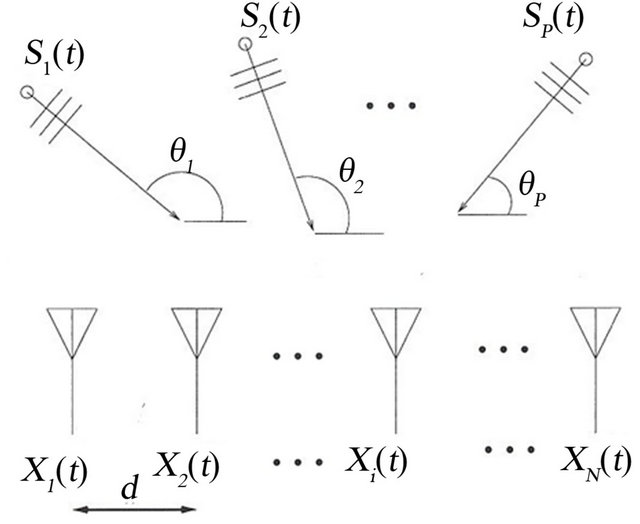
Figure 1. Receiving array and plane-wave arrivals.
exactly, however this difficulty can be overcome by using the standard MUSIC algorithm [5,6], which constitutes an angular pseudo-spectrum and an indicator of directions of arrival of different signals. The problem then reduces to estimating the signal powers from each of the P directions.
This study focuses on developing estimators which are used to identify the distribution of signal power generated by acoustic sources. This paper is organized as follows. An array signal model and the spatial covariance matrix of the sensor outputs are formulated in Section 2. The conventional beamformer and adaptive beamformers are presented respectively in Sections 3 and 4. A technique to obtain the strengths of signals arriving at an array of sensors based on the covariance vector of signals is developed in Section 5. A signal power estimation obtained by the pseudoinverse of the array manifold matrix is studied in Section 6. Numerical and experimental results showing the effectiveness and the weakness of different algorithms in signal power estimation are presented in Section 7. This paper is briefly concluded in Section 8.
2. Signal Representation and Sensor Output Covariance Matrix
Consider a uniform linear array with N sensors (Figure 1). Assume that P acoustical plane waves at frequency f impinge upon the array from P different directions . The complex envelope of the kth sensor’s output is [3-5]
 (1)
(1)
where the meanings of the various parameters are as follows:  is the complex envelope of the ith signal source at the first sensor; d is the space between two adjacent sensors;
  is the signal wavelength corresponding to frequency f and
  is the additive noise output of the kth sensor.
The complex envelope of the ith source is a zero-mean complex random variable. Its variance, denoted pi, characterizes the signal power of the ith source which we wish to estimate
 (2)
(2)
Here,  is the expectation operator and the superscript * represents the complex conjugate.
Equation (1) can also be expressed in the vector form as the N-dimensional vector [3]
 (3)
(3)
where

Here, T denotes transpose, and the direction of arrival of the ith signal source is represented by the N-dimensional complex vector . The noise is assumed to be spatially white (uncorrelated from sensor to sensor) and the same power level is present in each receiver. With these assumptions, the covariance matrix for the noise alone is given by
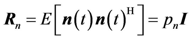 where
where  is the noise power,
  the
the  identity matrix and the superscript H denotes the Hermitian transpose operation. Equation (3) may be rewritten in the matrix form
 (4)
(4)
 is the
  array manifold matrix containing the manifold vectors for different sources as its columns,
 . For any single plane wave arrival, the outputs from the N individual receivers will differ in phase by an amount determined by the geometry of the array and the arrival direction. In other words, the elements Akr of the matrix A are known functions of the signal arrival angles and the array elements locations. It can readily be seen that the output signal from the qth sensor may be written as
 (5)
(5)
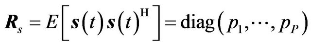
Since the P arrivals are by assumption independent, the source covariance matrix is given by
 (6)
(6)
and the diagonal elements are the powers of the sources , from the P directions, which we wish to estimate. The spatial covariance matrix of the receiver outputs can be expressed, for signals uncorrelated of each other and of noise, as
 (7)
(7)
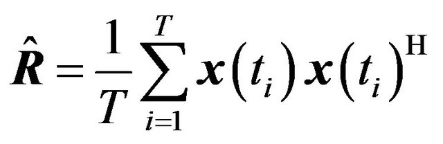
In practice, the spatial covariance matrix is estimated by a finite number of time domain samples (snapshots) and the following estimated form is used
 (8)
(8)
where  is the array signal vector sampled at time ti and T is the number of such samples. The caret (^) denotes an estimated value. We can now derive a variety of processors to estimate the strengths of P independent signals arriving at array of N sensors, when the arrival directions are known. Note that the number of sources can be obtained by examining the singular values of the covariance matrix [3].
3. Conventional Beamformer
The conventional beamformer, also called the “time delay and sum” or “unweighted add-squared” beamformer, consists of a system of delay and sum networks which are designed to make the signals from the beamformer direction in phase at each sensor. The directional data  from direction j must be estimated from the sensors output data vector
 . The usual approach is to find a matrix
 , such that
  reconstructs the directional data, and for a conventional beamformer the equation is [8]
 (9)
(9)
A power estimate for the signals can be found by forming the covariance matrix
 (10)
(10)
and the strength of the ith source estimated by the conventional beamformer is
 (11)
(11)
However, this leads to a biased estimate, as can be seen by substituting (7) into (10)
 (12)
(12)
So unless  and
and , neither of which is generally the case, then the estimate will be biased.
4. Minimum Variance Beamformer
The conventional beamformer can be considered as a kind of linear spatial filter with dataindependent coefficients. In contrast, the minimum variance beamformer, called also the standard Capon beamformer [3], can be considered has a kind of data-dependent spatial filter, in which the coefficients, represented by the weight vector w of the array element outputs, are chosen such that the filter has a constant gain at a particular direction ![]() while its output power is minimized. The constraint ensures that the signal power coming from the ith source will be reproduced in undistorted form in the processor output. Thus, the beamformer tries to eliminate as best it can all the signals received at the sensors except the signal coming from the ith wanted source. The weight vector w is selected so as to minimize the output power of the array
while its output power is minimized. The constraint ensures that the signal power coming from the ith source will be reproduced in undistorted form in the processor output. Thus, the beamformer tries to eliminate as best it can all the signals received at the sensors except the signal coming from the ith wanted source. The weight vector w is selected so as to minimize the output power of the array
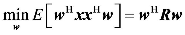 (13)
(13)
subject to the constraint
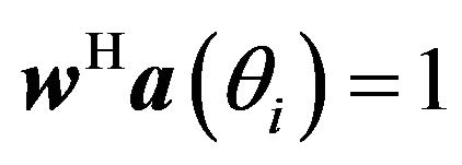 (14)
(14)
By the method of Lagrange’s multiplier, it can be shown that the optimum weight vector is
 (15)
(15)
and the power of the ith source estimated by the standard Capon beamformer is
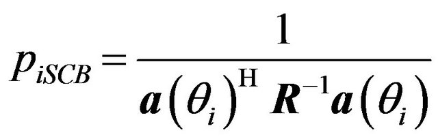 (16)
(16)
The standard Capon beamformer has better resolution than the conventional beamformer provided that the array steering vector corresponding to the signal of interest is accurately known. However, the performance of this traditional adaptive beamformer can degrade seriously in practice when errors exist in the signal of interest steering vector, which may be due to look direction error, array sensor position error and small mismatches in the sensor responses. In such cases the signal of interest might be mistaken as an interference signal and might be suppressed. A robust Capon beamforming algorithm [9], which is a natural extension of the standard Capon algorithm, is presented to overcome this difficulty. In the robust Capon beamforming algorithm we suppose that  is the true direction vector of the ith source,
  is the assumed direction of the ith source and we consider that
  is in the vicinity of
 . This can be expressed mathematically by the following inequality:
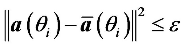 , where
 ![]() is a bound controlling the uncertainty in the assumed look direction. To derive the robust Capon beamforming algorithm we use the reformulation of the standard Capon beamforming problem to which we append the previous inequality. We have the following minimization problem
is a bound controlling the uncertainty in the assumed look direction. To derive the robust Capon beamforming algorithm we use the reformulation of the standard Capon beamforming problem to which we append the previous inequality. We have the following minimization problem
 (17)
(17)
subject to the constraint
 (18)
(18)
The optimization problem can be rewritten as the following form
 (19)
(19)
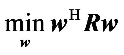
subject to the constraint (18). We consider the solution on the boundary of the constraint set and we reformulate the optimization problem as the following quadratic form with a quadratic equality constraint
 subject to
  (20)
(20)
This problem can be solved by the method of Lagrange’s multiplier which is based on the cost function
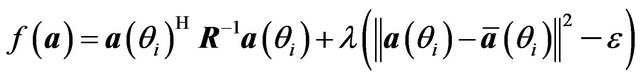 (21)
(21)
Differentiating (21) with respect to  and equating to zero gives the optimal solution
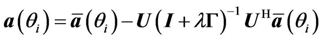 (22)
(22)
where  and
and ![]() are
are  matrices containing the eigenvectors and eigenvalues of the covariance matrix
  and
and ![]() is the Lagrange multiplier. Using (22) in the equality constraint of (20) the Lagrange multiplier is obtained as the solution to the constraint equation
is the Lagrange multiplier. Using (22) in the equality constraint of (20) the Lagrange multiplier is obtained as the solution to the constraint equation
 (23)
(23)
The signal power estimation of the ith source using the robust Capon beamformer is then
 (24)
(24)
In summary of this section, the standard Capon beamformer is an optimal spatial filter that maximizes the signal to noise ratio, provided that the true covariance matrix and the array steering vector are accurately known. However, the covariance matrix can be inaccurately estimated due to imperfect array calibrations, gain and phase errors in the sensors. The robust Capon beamformer presented in the paper can then be used in such situations for both signal power estimation and source location as shown in examples given in Section 7. Another power estimator using the covariance vector of signals is presented in the next section.
5. Signal Power Estimation by the Covariance Vector Estimator
Since we are interested in the signal powers, the covariance matrix of the data contains all the information about these signal strengths. The correlation between sensor k and l is  and from Equation (5) we obtrain
 (25)
(25)
But since signals from different directions must be uncorrelated, we have
 (26)
(26)
The sensor noise power on each sensor is constant and equals pn and  for
for  and zero otherwise. Equation (26) may be split into real and imaginary components as
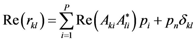 (27)
(27)
 (28)
(28)
Of the 2N2 equations represented by (27) and (28) only  equations are independent. Indeed, one gets
 (29)
(29)
 (30)
(30)
 (31)
(31)
Equations (27) and (28) may then be written in the form
 (32)
(32)
where r, B and p are reals. r is the  vector which contains the real and imaginary components of
  and is called the covariance vector; p is the
  vector containing the signal powers
  and sensor noise power pn. Note that if the sensor noise is small, it may be desirable to omit the model of sensor noise. B is the
  matrix which contains all the array geometry terms and
  if required
 (33)
(33)
The least squares solution to (32) is given by
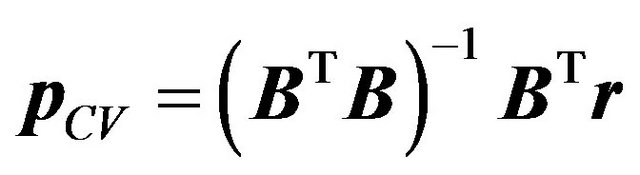 (34)
(34)
pCV is the vector containing the strengths of signals by the covariance vector. Performances of this estimator are given in Section 7. Another power estimator based on the pseudoinverse of the array manifold matrix A is presented in the next section.
6. Signal Power Estimation by the Pseudo-Inverse of the Array Manifold Matrix
From Equation (7) we obtain
 (35)
(35)
A possible approach to estimate the signal strengths is to select the P diagonal elements of the matrix Rs. We get
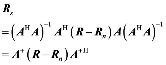 (36)
(36)
where A+ is the pseudoinverse of the array manifold matrix. To obtain the noise covariance matrix , or the noise power pn, we consider the eigenvalue decomposition of the covariance matrix R
 (37)
(37)
The rank of  is equal to the number of incident signals P and can be determined from the P largest eigenvalues of R. The minimum eigenvalue of R corresponds to the noise power pn.
Numerical simulations and experimental tests are now presented to evaluate the performances of the estimators presented in the paper.
7. Numerical and Experimental Results
The conventional beamformer (CB), the standard Capon beamformer (SCB), the robust Capon beamformer (RCB), the covariance vector estimator (CV) and the pseudoinverse estimator (PI) are employed to estimate the strengths of signals arriving at an array of receivers. In our simulations, we assume a uniform linear array with N = 6 omnidirectional sensors and half-wavelength sensor spacing. Four point sources are located at bearings of— 30˚, 0˚, 22˚ and 45˚. The source powers are respectively 60 dB, 55 dB, 80 dB and 70 dB and the number of snapshots is T = 4096. The signal to noise ratio is SNR = 20 dB. Figure 2 shows the power estimates of CB, SCB and RCB as a function of the direction angle in the case where there are no gain and phase errors in the sensors of the array. The small circles denote the true direction of arrival and the true power of the four sources. The SCB and RCB estimators provide excellent power estimates of the incident sources and can also be used to determine their directions of arrival based on the peak power loca-

Figure 2. Power estimates versus the steering direction θ using CB, SCB and RCB without gain and phase errors and SNR = 20 dB.
tions. The CB estimator has much poorer resolution than both SCB and RCB and the sidelobes of the former give false peaks and false directions of arrival of sources.
Figure 3 shows the power estimates of CB, SCB and RCB in the case where there are a gain error of 0.02 and a phase error 0.2˚ in each sensor. We note that SCB and RCB can still give good direction of arrival estimates for the incident signals based on the peak locations, however, the SCB estimates of the incident signal powers are way off. In this case, only the RCB algorithm gives good power estimates of the incident sources and can also be used to determine their directions of arrival based on the peak locations.
The remaining part of the section is focused on the application of the developed algorithms to the experimental identification of noise sources generated by two loudspeakers. The experimental setup is schematically shown in the block diagram of Figure 4 with the acoustic array and two sources (the loudspeakers) in the anechoic room.

Figure 3. Power estimates versus the steering direction θ using CB, SCB and RCB with 0.02 gain error and 0.2˚ phase error in each sensor and SNR = 20.
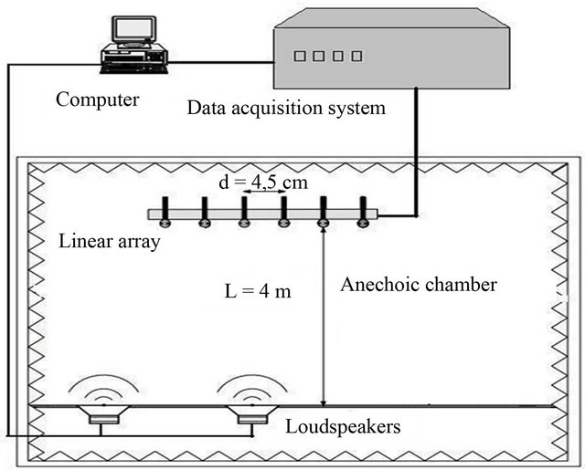
Figure 4. Block diagram of the experimental system.
The receiving acoustic array is linear and formed with six omnidirectional microphones equally spaced, with inter-element spacing of d = 4.5 cm. The two acoustic sources (the loudspeakers) and the acoustic array are in the same horizontal plane. The transmitting loudspeakers generate two typical audio signals at a frequency of 3800 Hz corresponding to a microphone separation distance of one-half wavelength. The number of snapshots is T = 4096. We are able to find the direction of the two sources by using the MUSIC algorithm, however, unlike the methods mentioned earlier, MUSIC does not physically correspond to the signal power. The MUSIC algorithm is only an indicator of directions of arrival of different signals. Figure 5 shows the normalized angular spectrum function obtained from MUSIC where important peaks appear at the signal directions. We obtain the angular position of the sources  and
and .
.
Once the arrival angles have been determined we can estimate the power of the two acoustic sources by our proposed algorithms. Table 1 shows the results obtained by our algorithms.
The experimental results confirm that the CV and the PI estimators give very similar results and the RCB estimator overestimates very slightly the source powers.
Figure 6 shows the power estimates versus the steering direction using the RCB algorithm. From this plot we obtain simultaneously an estimate of directions of arrival and an estimate (slightly overestimated) of the power of the two sources, based on the two peak locations.
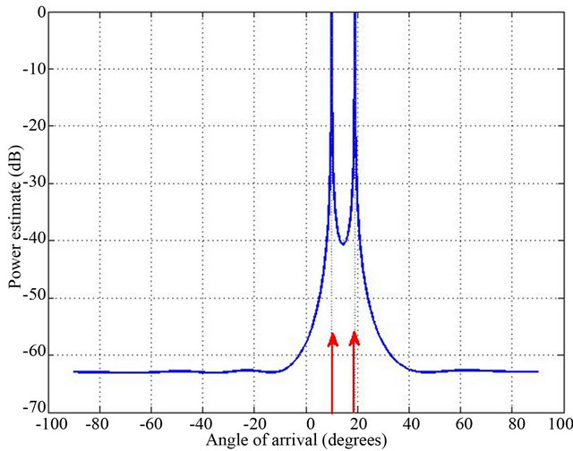
Figure 5. Experimental MUSIC spatial spectra.
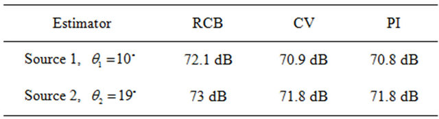
Table 1. Power estimation using different estimators.
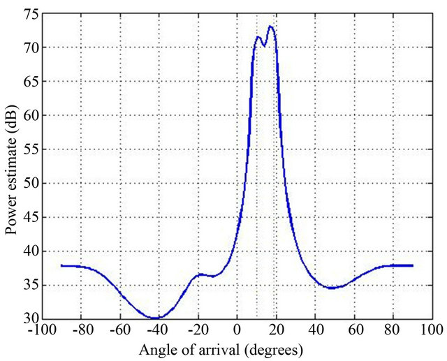
Figure 6. Experimental robust capon beamformer.
8. Conclusions
Five signal processors to estimate the strengths of signals arriving at an array of sensors have been studied. The conventional beamformer and the standard Capon beamformer provide in general poor power estimates of the incident sources. The robust Capon beamformer gives good power estimates and can also be used to determine the directions of arrival of incident sources. The covariance vector and the pseudoinverse estimators give excellent power estimates. From numerical simulations and field tests, the RCB, CV and PI algorithms exhibit remarkable effectiveness in finding the strengths of signals. The performances of these algorithms in the case of very close sources are under investigation.
These techniques have been developed for the estimation of signal strengths using an array of receivers. However, the principles can be applied to a wide range of other estimation problems, of which the spectrum analysis of a time series is an example.
REFERENCES
- F. J. Fay, “Sound Intensity,” Elsevier Applied Science, Amsterdam, 1989.
- M. R. Bay, “Application of BEM-Based Acoustic Holography to Radiation Analysis of Sound Sources with Arbitrarily Shaped Geometries,” Journal of the Acoustical Society of America, Vol. 92, No. 1, 1992, pp. 533-549. doi:10.1121/1.404263
- P. Stoica and R. Moses, “Spectral Analysis of Signals,” Prentice Hall, Upper Saddle River, 2005.
- T. J. Shan, M. Wax and T. Kailath, “On Spatial Smoothing for Direction of Arrival Estimation of Coherent Signals,” IEEE Transactions on Acoustic, Speech and Signal Processing, Vol. 33, No.4, 1985, pp. 806-811. doi:10.1109/TASSP.1985.1164649
- R. O. Schmidt, “Multiple Emitter Location and Signal Parameter Estimation,” IEEE Transactions on Antennas and Propagation, Vol. 34, No. 3, 1986, pp. 276-280. doi:10.1109/TAP.1986.1143830
- P. Stoica, Z. Wang and J. Li, “Extended Derivation of MUSIC in the Presence of Steering Vector Errors,” IEEE Transactions on Signal Processing, Vol. 53, No. 3, 2005, pp. 1209-1211. doi:10.1109/TSP.2004.842201
- M. Yang, M. Al-Kutubi and D. T. Pham, “In-Solid Acoustic Source Localization Using Likelihood Mapping Algorithm,” Open Journal of Acoustics, Vol. 1, 2011, pp. 34-40. doi:10.4236/oja.2011.12005
- H. A. d’Assumpcao an G. E. Mountford, “An Overview of Signal Processing for Arrays of Receivers,” Journal of Electrical and Electronics Engineering, Vol. 4, No. 1, 1984, pp. 6-18.
- J. Li, P. Stoica and Z. Wang, “Robust Capon Beamforming,” IEEE Signal Processing Letters, Vol. 10, No. 6, 2003, pp. 172-175. doi:10.1109/LSP.2003.811637