Open Journal of Acoustics
Vol.2 No.3(2012), Article ID:22602,9 pages DOI:10.4236/oja.2012.23011
Ultrasound Imaging of Spinal Vertebrae to Study Scoliosis
1Departmentof Biomedical Engineering, University of Alberta, Edmonton, Canada
2Department of Radiology and Diagnostic Imaging, University of Alberta, Edmonton, Canada
3Department of Surgery, University of Alberta, Edmonton, Canada
Email: wei.chen@ualberta.ca, lawrence.le@ualberta.ca, *elou@ualberta.ca
Received July 21, 2012; revised August 19, 2012; accepted August 28, 2012
Keywords: Ultrasound; Cobb Angle; Phased Array; Scoliosis; Spinal Deformity; Ultrasonic Imaging
ABSTRACT
Scoliosis is a musculoskeletal disorder manifested as a three-dimensional spinal deformity. It affects 2% - 3% of the adolescent population. The conventional method to diagnose scoliosis is to measure the Cobb angle from posteroanterior radiograph. Since radiation exposure is not desirable for patients, other non-ionizing methods have been explored. Among all the non-ionization methods, ultrasound (US) is a potential cost-effective method. However, our understanding of US interaction with the vertebrae or the spine is limited. The purpose of this study was to demonstrate the ability of US to identify bony landmarks for measuring spinal deformity. This study used a phased array US system with a 5 MHz transducer and a position encoder. In-vitro experiment on a cadaver vertebra and a pilot clinical study were carried out. The in-vitro experimental results showed that the lamina and spinous process were strong reflectors from the single vertebra. Less than 4% of error occurred on the dimension measurements. The pilot study was performed on a healthy subject and a scoliotic patient. The results indicated the lamina and spinous process could be identified and the curvature of the spine could be estimated using the reflectors. The difference of the curvature angle of the spine measured from the radiograph and the US images was 2˚. These results have illustrated that US is a promising tool to measure curvature of spinal deformity and study scoliosis.
1. Introduction
Scoliosis is a complex three-dimensional (3D) deformity of the spine associated with vertebral rotation [1]. The curvature affects the rib cage and presents as deformities of the trunk. Approximately 80% of the cases are known as idiopathic scoliosis (IS) for which there is no known cause. The prevalence of IS in the childhood and adolescent population ranges from 0.5% to 3% [2] and is more common in girls than boys. The ratio of girls to boys is 8:1 for patients requiring treatment [3]. The previous surveys [4-7] reported that patients with scoliosis suffered higher mortality, more common backaches, decreased physical capacity, and the deteriorated pulmonary function, which negatively affect the quality of life.
The most commonly used method to diagnose adolescent idiopathic scoliosis (AIS) is to measure the spinal curvature from a posteroanterior (PA) radiograph. The curvature angle is called the Cobb angle measured by the Cobb method [8]. Although the Cobb angle is the gold standard to measure the severity of scoliosis and can be used to predict its progression, the measurement is limited to two-dimension which does not adequately quantify the 3D spinal deformity. Besides the spinal curvature, vertebral rotation is another useful parameter to describe the full extent of scoliosis [1] and evaluate the treatment outcome [9]. Several methods have been developed to measure vertebral rotation on radiographic images [10-12] and computed tomography (CT) images [13,14].
X-ray based techniques expose patients to harmful ionizing radiation and CT scanners emit more radiation than conventional radiography. Young scoliotic patients require years of follow-up to monitor the progression of spinal curvature with the possibility of accumulating more radiation doses due to increasing number of radiographic exposures. Some cohort studies involving female patients showed frequent exposure to radiation during childhood and adolescent may increase breast cancer risk [15,16]. Therefore, alternative non-invasive, radiationfree, and reliable methods to study scoliosis are urgently sought. Magnetic resonance imaging (MRI) could reconstruct high-quality tomographic images of spinal vertebrae [17,18]. However, the use of MRI is costly and time consuming; therefore, its use to evaluate AIS still remains very limited.
Surface topography is a 3D measurement of back’s surface using scanned light, photographic techniques or sensors [19]. Several systems based on surface topography were suggested such as optical based Moire fringe topography, the integrated shape imaging system, ISIS (Oxford Metrics, Ltd., Oxford, UK), and the Quantec Spinal Imaging System, QSIS (Quantec Inc., Lancashire, England) [20-23]. For the past decade, researchers have focused on the full torso study. A patented INSPECK system [24] and a commercial non-contact 3D digitizer (Vivid 910, Konica Minolta, Japan) have been used to capture the full torso and tried to correlate the surface features with internal alignment [25,26], but the correlation was not strong.
Another method, which used the sensor of the Ortelius 800TM system (Orthoscan Technologies Inc., MA, USA) to touch the spinous processes of the scoliotic patients, was able to reconstruct the spinal alignment and to calculate the vertebral locations and the curvature angles. A study involving 52 AIS patients showed good agreement between the curvature angles from the Ortelius and the Cobb angle measurements [27]; however, a recent study [28] did not support the previous findings.
Among the aforementioned methods, ultrasound (US) is the most attractive method as it is cost effective, portable, easy to operate, and has no radiation risk. The tissue-bone interface is a strong reflector and reflects most of the US signals [29], thus making vertebral imaging possible. Using a medical US scanner (Shimazu SDL- 300) with a 5.0 MHz transducer, researchers from Kyoto University were able to identify the transverse processes and the laminae in 47 patients in prone position [30]. They also measured spinal rotation and found that the Cobb angle and the vertebral rotation had a linear correlation in untreated patients. Another study [31] showed that the US could locate the lumbar intervertebral level accurately. Recently, Li et al. [32] demonstrated that US could be used to trace the spinous process during brace fitting process and to calculate the spinous process angle (SPA). High correlation was obtained between the Cobb angle and SPA in 12 AIS patients [32]. However, another study reported the SPA underestimated the severity of a scoliotic curve compared with Cobb angle [33]. The contradictory results between [32] and [33] were due to the fact that the ranges of Cobb angle under investigation were significantly different: smaller range (15˚ - 29˚) in [32] and larger range (20˚ - 75˚) in [33]. More studies are required to confirm a reliable correlation between the SPA and Cobb angles. Studies of scoliosis using US are limited. While the literature has, so far, concluded positively the potential of using US to assess scoliosis, the evidences presented in those reports are, quite regrettably, very few. There is a lack of good quality US images and convincing discussion of the image features with reference to the US reflectors or markers of the vertebra. In an effort to advance the research of using US to study sco liosis, it is important to be able to interpret the US images of the spine with confidence. To accomplish this, confirming an existence of a good correlation between the features of the US images and those of the vertebrae is crucial.
In this paper, we studied the US images of spinal vertebrae from both the in-vitro experiment and a pilot clinical trial using a non-medical US scanner. The objective is to relate the features of the US images to the source of the echoes recorded on the plane of acquisition. Ultimately, we hope to identify suitable US markers for the assessment of scoliosis.
2. Methods
2.1. Vertebra Phantom
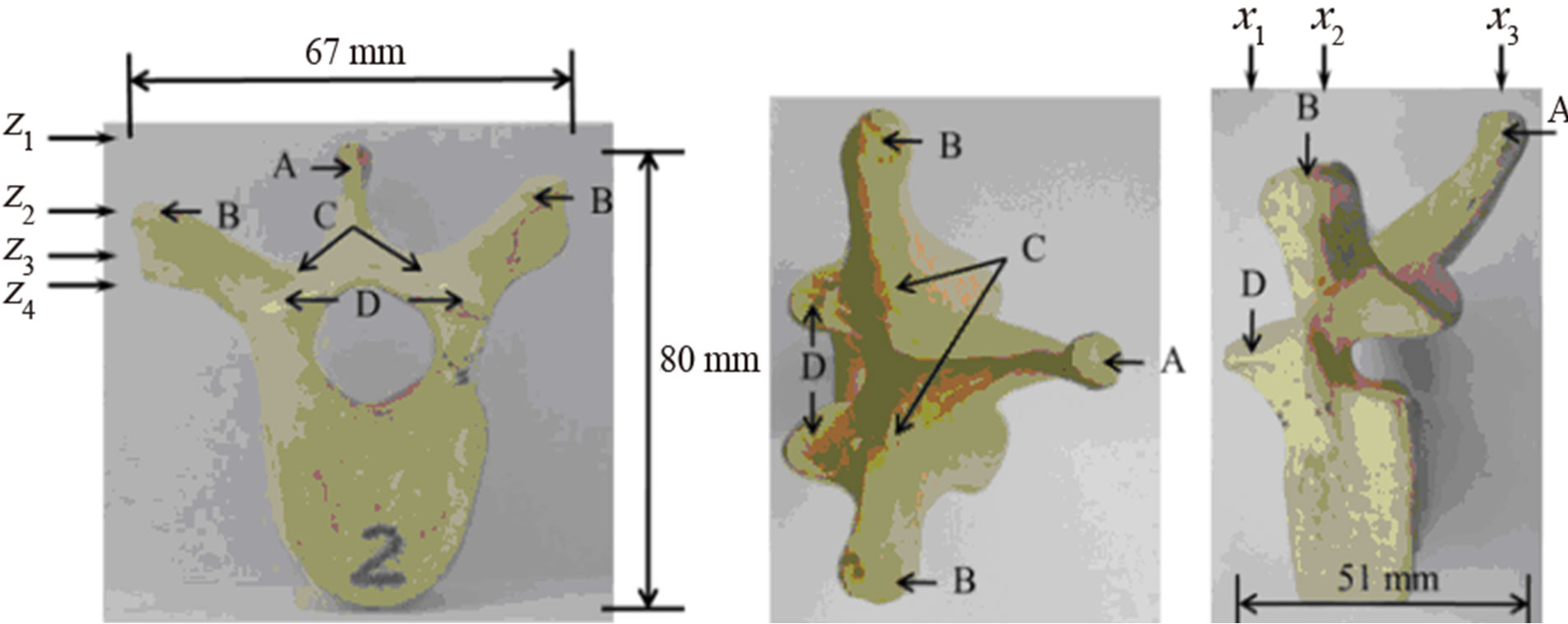
A cadaveric thoracic vertebra (T9) phantom was used in this experiment. Figure 1 shows the front, top, and side views of the vertebra. With soft tissue removed, the specimen was cleaned, dried, and treated for preservation and frequent handling. The major posterior arch structures of the vertebra, which include the spinous process (SP), transverse process (TP), laminae, and superior articular process (SAP), are identifiable from the images (Figure 1). The maximum length, height, and width of the vertebra are 67 mm, 80 mm, and 51 mm respectively.
2.2. Clinical Study
A healthy and non-scoliotic female volunteer, who is a team member from our laboratory, consented to participate in the pilot clinical study. The second subject was an AIS patient, 11-year old female, with main thoracic curve between T5 and T12 vertebrae (Cobb angle 29˚), treated by bracing and had no in-brace radiograph taken on the same day of the study. Consent was also obtained from this patient.
 (a) (b) (c)
Figure 1. The vertebra phantom: (a) front view, (b) top view, and (c) side view. The letters A, B, C, and D indicate the positions of the spinous process (SP), transverse process (TP), lamina, and superior articular process (SAP) respectively. The X-arrows (x1-x3) show the positions of the displayed images presented later in Figure 4 while the Z-arrows (z1-z4) show the positions of the displayed images presented later in Figure 6.
2.3. Ultrasound Equipment
In this study, we used an Olympus TomoScan Focus LTTM Phased Array Ultrasound system (Olympus NDT Inc., Canada) as shown in Figure 2(a). Beam forming and transmit/receive focusing for different depth zone can be achieved by applying time delays among transducer elements. The scanning pattern can be linear or sectorial (or angular). The US system is connected to a computer via Ethernet port. The computer with the TomoviewTM software (Version 2.9 R6) installed is used to control the data acquisition process and modify the parameters of the US beam such as scanning mode, beam angle, focal position, and active aperture. The acquired data can be exported to the computer for further post-acquisition analysis. Realtime data compression and signal averaging are also available.
The US transducer used was a 5.0-MHz 64-element array probe (5L64-I1) (Figure 2(b)). The probe has an active area of 38.4 mm (length) by 10 mm (elevation) with a pitch (p) of 0.6 mm. For transmit focusing, the outer elements are fired before the inner elements to achieve depth focusing. Increasing time delays between adjacent elements decreases focal depth while reducing the delays causes distal depth focusing. For receive focusing, the echoes coming back from a certain depth are stored, delayed, and then summed to produce an US signal. Generally, the echoes received by the outer elements travel longer distances than the echoes by the inner elements. In order to align the echoes for summing, the echoes received at the center element of the group are delayed the most while those received at the edge of the groups are delayed the least. The amount of delay is such to ensure the phases of the echoes are aligned to be summed.
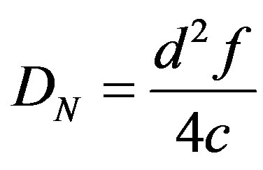
We chose to use a group of twelve elements for depth focusing because of the compromise between depth penetration and frame size. The maximum focal depth, DN for the 12-element group is 43.7 mm according to the following equation [29]:
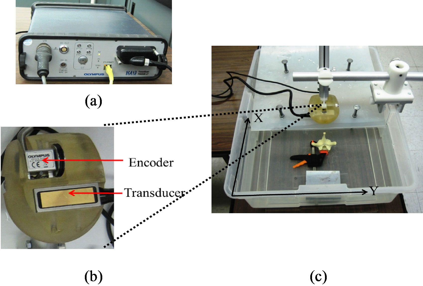
Figure 2. Experimental equipment and setup: (a) the TomoScan Focus LTTM phased array ultrasound system, (b) the holder with the mini-wheel encoder and transducer, and (c) the experimental setup.
 (1)
(1)
where the active group aperture, d is 7.2 mm (12 × p), the frequency, f is 5 MHz, and the speed of sound, c is 1480 m/s for water [34]. The beam converges at the focal depth where the beam width is the minimum, providing the best lateral resolution and beyond which the beam starts to diverge. Lateral resolution is depth dependent. The TomoScanTM system has the dynamic depth focusing (DDF) capability, which is a beam forming technique to extend the lateral resolution over a depth range. We considered linear scanning with DDF. Based on our resolution phantom study, the lateral resolution remains constant 1.2 mm at depth between 5 mm and 43.7 mm with a 12-element group. The encoder (Figure 2(b)) works in synchronization with the transducer movement during data acquisition. The position coordinates of the transducer are recorded by the system.
2.4. Experimental Setup
The vertebra phantom rested at the bottom of a small water tank (Figure 2(c)) with the transverse processes at the same horizontal level to minimize vertebral rotation. A 2 mm thick polypropylene sheet with an US speed of 1628 m/s, calculated by the pulse-echo method [29], was used to mimic the skin. The sheet was supported by screws and placed about 7 mm above the spinous process of the phantom. The tank was filled with water until it just covered the sheet. The human skin thickness varies between 1.55 mm and 2.54 mm [35] with an average US speed 1645 m/s for epidermal layers and 1595 m/s for dermal layers respectively [36]. Therefore, the polypropylene sheet is an appropriate skin mimics. Water has an US speed of 1480 m/s similar to 1540 m/s of soft tissue and was used to simulate the soft tissue. The whole experimental setup was to mimic the human back including skin, soft tissue, and vertebra.
The transducer and the encoder were placed in a holder (Figure 2(b)). The holder was mounted to an aluminum vertical arm. An aluminum guidance device or glider was mounted to the edge of the water tank (Figure 2(c)). The glider, which slid along the edge, has a horizontal arm, to which the holder arm was firmly attached. The horizontal arm was engraved in metrics to indicate the y-position of the holder. During scanning, one held the holder arm and moved the glider forward along the x-direction with a speed of no more than 5 mm/s. Among other factors, the speed depended on the depth of interest because longer listening time was required for the transducer to record echoes from deeper depth. At speed faster than 5 mm/s, the encoder wouldn’t trigger the transducer to fire, causing no transmitting signals and thus null or dead US image; speed slower than this value increased the scanning time.
For the pilot study, a custom frame was built with a track to allow the holder of the transducer and encoder to move vertically. Each participant wore a gown with an open back during the scanning process. The participant sat straight inside the frame and looked straight with arm resting on a metal bar at the front and chest level. This set up was to minimize the sway of subjects’ bodies. The operator move the holder vertically along the back scanning from T4 to L4 for the volunteer and T5 to L4 for the AIS patient. The transducer was slightly pushed against the back tissue with ultrasound gel between the transducer and the skin to ensure good coupling.
2.5. Data Acquisition and Processing
For ease of discussion, we defined an XYZ-coordinate system as shown in Figure 3. The probe moved along the X-axis. A 12-element group defined an A-line. Each A-line was 7418-point long separated by 0.01 µsec interval. Since each group was shifted by one element interval, the spacing between A-lines was 0.6 mm. A maximum of fifty-three A-lines formed an image or frame with an effective aperture 31.2 mm. Each frame was a 2D transverse view of the vertebra in the Y-Z plane (perpendicular to the X-axis). To convert the temporal interval Dt to depth interval Dz, one would divide Dt by 2 to account for the two-way travel time of the US and multiply it by 1480 m/s. The resultant depth interval was 0.0074 mm. At a 5 mm/sencoder speed, the spacing interval between frames was 1 mm. Signal averaging and data compression were not applied.
Since the length of the phantom was longer than the effective aperture of the transducer array, each frame acquired by one scan didn’t cover the whole length of the vertebra phantom. Thus, three scans were required to cover the whole vertebra. A 70 mm × 81.2 mm area on the XY-plane defined the scanning area for the vertebra phantom. After finishing a scan along the X-axis, the holder was translated back to the beginning of the scan and moved along the Y-axis to a new index-position for the new scan. The starting (x, y) positions of each scan
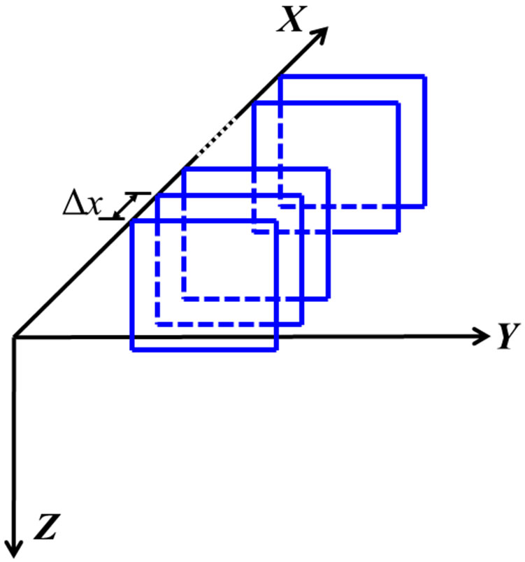
Figure 3. The coordinate system: X is the scanning axis, Y is the axis for element index, and Z is the depth axis. The squares represent the acquired frames. The spacing between frames is Dx.
were recorded; the multiple scan files were merged to form a single data file of the whole phantom using the TomoviewTM software. When the overlapped data was merged together, the intensity of the resultant voxel was assigned using maximum intensity projection (MIP) method [37]. The merged data had a depth resolution of 0.074 mm after 10-folded decimation. Hereafter, a frame was referred to a merged frame. For the in-vivo study, two scans were required to cover the body size of the volunteer while one scan was adequate for the AIS patient.
The data was further reconstructed to form the sagittal and coronal views on the XZ-plane and XY-plane respectively. The images could be displayed either by single slice or by merging the contiguous slices with varying slice thickness. The images were displayed with 16 colors where the red color was for hyper-echoic area, blue for hypo-echoic, and white for anechoic. The other colors were linearly interpolated.
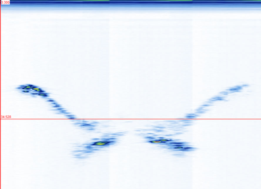
3. Results Three frames obtained at three scanning positions x1, x2, and x3 (indicated in Figure 1(c)) are shown in Figures 4(a)-(c). The images show the SAP, TP, laminae, and SP in their respective frames. There are 51 frames traversing the width of the vertebra. Their projections on the YZ-plane provide an overall comparison of the echo strength from the vertebral structures (Figure 4(d)). The image shows a general shape of a “W” as compared with the front view of the vertebra (Figure 1(a)). The echoes from the SP and laminae are relatively strong while those from the TP and SAP are weak. The projections of all the sagittal images on the XZ-plane also display similar observations about their relative reflections from the laminae and SP (Fig
 (a)
(a)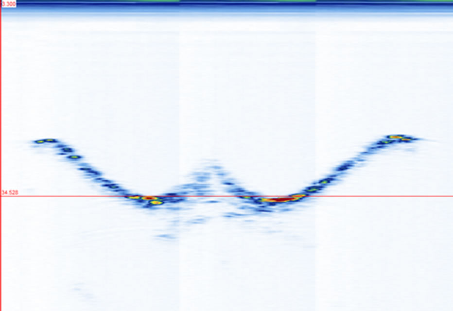 (b)
(b)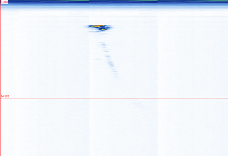 (c)
(c)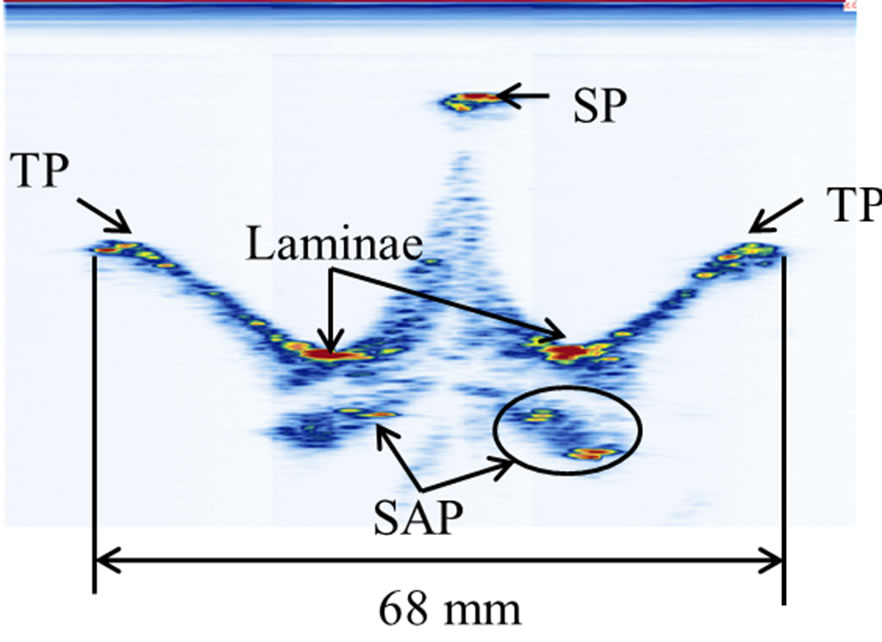 (d)
(d)
Figure 4. The transverse views of the vertebra phantom at different scanning positions as indicated in Figure 1(c): (a) at x1, (b) at x2, (c) at x3, and (d) the stacking of 51 frames. The red lines in (a)-(c) indicate the same depth level around z3.
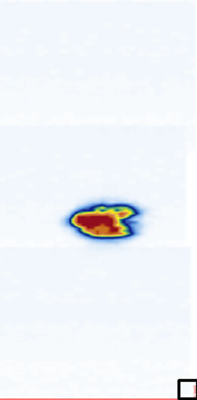
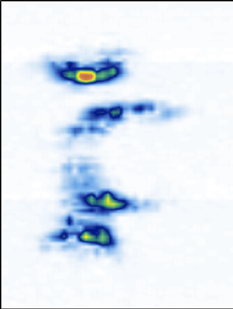
ure 5). The coronal views are shown in Figure 6 at four different depths: z1, z2, z3, and z4 as indicated in Figure 1(a). The 2D images are displayed with different slice thickness. Due to the uneven surfaces and curvature of the structures, thicker slices are necessary to delineate the structures and enhance the echo strength. The number of slices (equivalent thickness) used are 28 (2.07 mm), 24 (1.78 mm), 20 (1.48 mm), and 74 (5.48 mm) for the SP, TP, laminae, and SAP respectively. Figure 6(e) displays a coronal image formed by stacking all cross sectional images from the top of the SP to the bottom of the SAP, covering about 38 mm thick of the vertebra.
We have previously mentioned that thicker slices are necessary to image the structures with good confidence. To illustrate the point, we used a series of coronal images of the laminae for five different thicknesses ranging from 0.074 mm thick (1 slice, Figure 7(a)) to 1.48 mm (20 slice, Figure 7(e)). Starting at depth z3, a single slice image (Figure 7(a)) hardly reveals the laminae’s locations. A 5-slice image (Figure 7(b)) starts to display
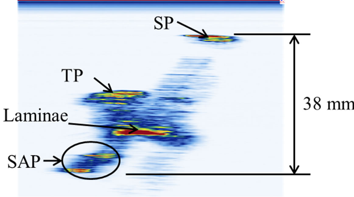
Figure 5. The projection of all sagittal images on the XZplane.
 (a)
(a)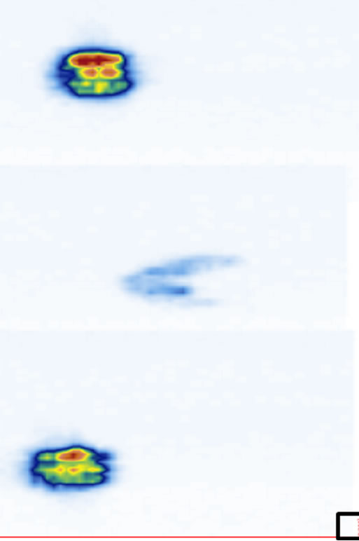 (b)
(b)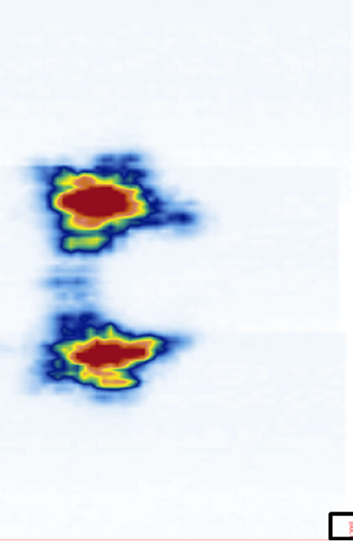 (c)
(c)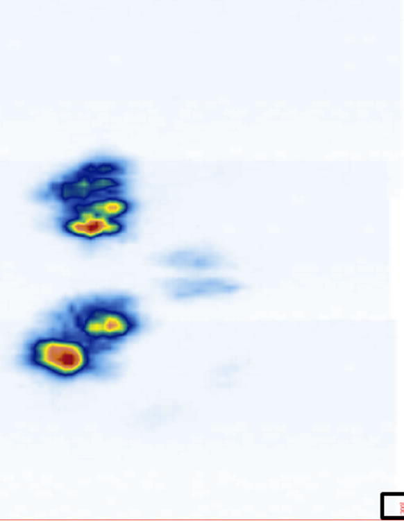 (d)
(d)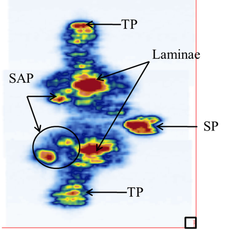 (e)
(e)
Figure 6. The reconstructed coronal views at different imaging depths showing different structures of the vertebra: (a) SP (at z1), (b) TP (at z2), (c) laminae (at z3), (d) SAP (at z4), and (e) image stacking from the top of the SP to the bottom of the SAP. The square at the southeast corner of each image is used as a point of reference.
their locations. A 10-slice image (Figure 7(c)) significantly improves the visibility of the laminae. A 15-slice thick image (Figure 7(d)) improves the image marginally. There is no visual difference between the 15-slice and 20-slice images. To determine the optimal number of slices, we referred to the transverse and sagittal images. By measuring the apparent thickness of the hyper-echoic area corresponding to the laminae from the sagittal view (Figure 5), we estimated 20 slices to be sufficient.
We further compared the dimensions of the structures using measurements from both the phantom and its corresponding US images. Three dimensions: The length of lamina centers, the length of the TP centers, and the length of the vertebra, were obtained from the transverse and coronal images; the height between them were taken from the transverse and sagittal images using the top edge of each structure. A digital caliper was used to measure the vertebra phantom while the dimensions of the US images were measured on the monitor using TomoScanTM measuring software. The centers of the features were used for the measurements and each measurement was repeated three times. The means and standard deviations of the measurements are listed in Table 1. The means are different by less than 1 mm (<4%).
For the in-vivo study, we performed a preliminary experiment on the volunteer. A transverse image of the thoracic vertebra T4 is shown in Figure 8(a) with a stacked image (11 slices) shown in Figure 8(b). The reflected signals from the heterogeneous soft tissues are strong. The top part of the white area in the middle of the image is the SP location. Underneath the SP is the shadow zone where no US reflections are recorded. The hyper-echoic areas on both sides of the SP are the laminae. However, it is difficult to locate the exact locations of the TP since
 (a)
(a)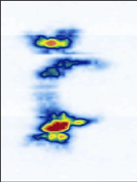 (b)
(b)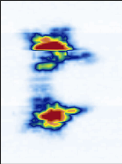 (c)
(c) (d)
(d) (e)
(e)
Figure 7. The reconstructed coronal views of the laminae of different thickness: (a) 0.074 mm (1 slice thick), (b) 0.37 mm (5 slices thick), (c) 0.74 mm (10 slices thick), (d) 1.11 mm (15 slices thick), and (e) 1.48 mm (20 slices thick).
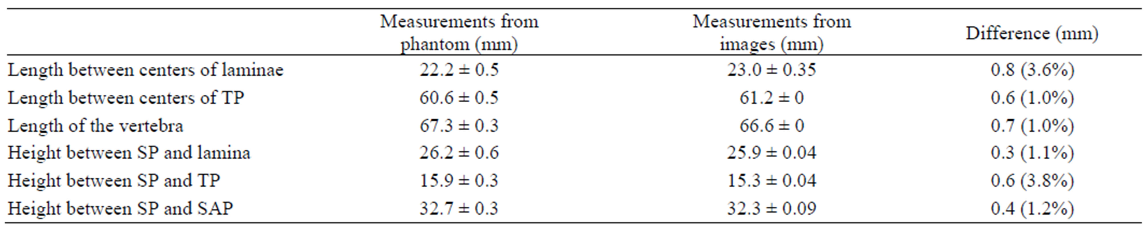
Table 1. Comparison of measurements between phantoms and images.
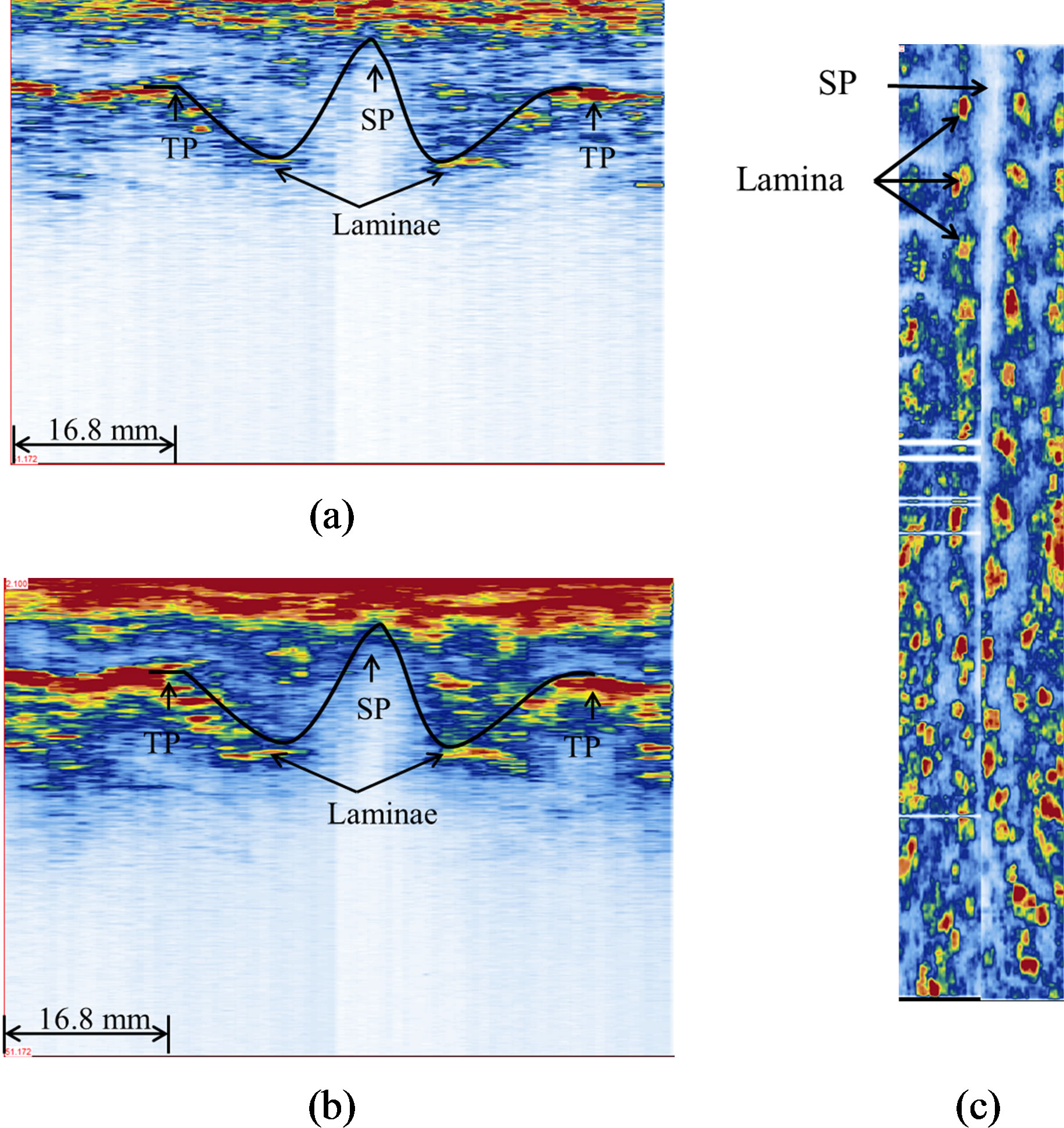
Figure 8. Ultrasound images of the healthy volunteer: (a) a transverse view (single frame), (b) a transverse view of 11 stacked frames, and (c) a coronal view (320 slices). The black curves in (a) and (b) outline the W-shape of a vertebra.
their reflections are interfered by the reflections of the overlying ribs. However the general W-shape can be recognized. From the coronal image shown in Figure 8(c), the SP and laminae can be identified and reflect a straight spine of the volunteer.
Figure 9(a) shows the PA radiograph from the AIS patient with the Cobb angle measured from T5 to T12. Figure 9(b) shows the US coronal image of the same patient, where the laminae (red area) and SP shadow zone (white area between laminae) can be recognized. To measure the coronal curvature from the US image, the center of lamina (COL) method is used. Two lines were drawn through the center of laminae at the levels of T5 and T12 to form the curvature angle. The angle measured from this US image was 27˚ and it was 2˚ different from the x-ray measurement. A transverse image from T6 is shown in Figure 9(c), in which the pair of laminae is not at the same level, which means there is an axial rotation on this vertebra. Even though an axial rotation occurred, the SP and laminae could still be identified as part of the W-shape.
4. Discussions
Ultrasonography has been a successful diagnostic imaging technique of choice to image soft tissues. Recently, US elastography has been used to retrieve the mechanical properties of soft tissue. Bone imaging using US is not common, but it has been shown that ultrasound can image bone [38-40]. When US encounters an interface separating two media of different acoustic impedance , there is a partition of energy at the interface. The amount of reflected energy very much depends on the impedance contrast (normal incidence):
 (2)
(2)
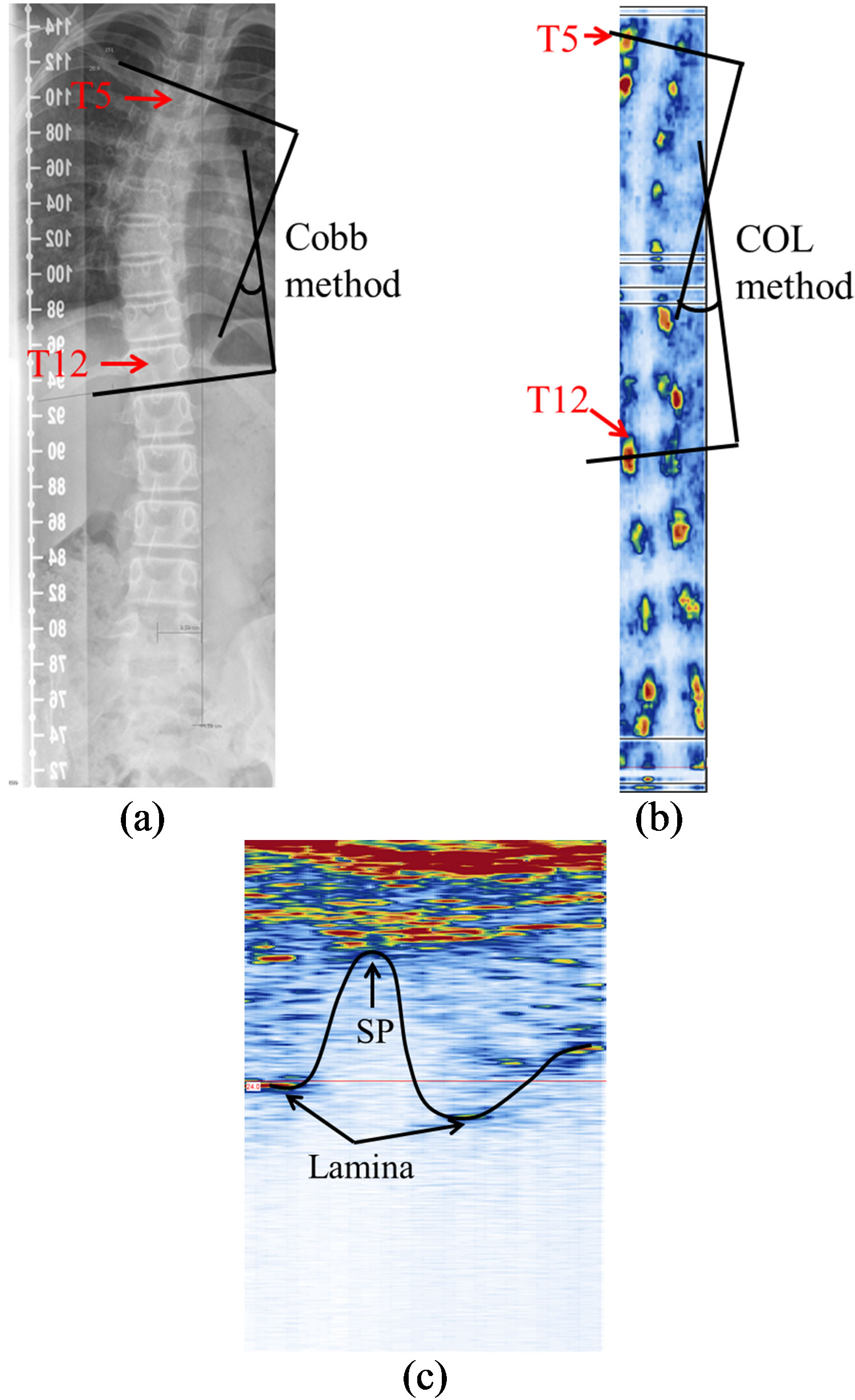
Figure 9. The spinal images of the AIS participant: (a) the PA radiograph; (b) the US coronal view (170 slices); and (c) a transverse image of a vertebrae (single frame).
Soft tissue-bone interface is a strong reflector. Considering the impedances of bone and soft tissue around 7.8 × 10⁻⁵ rayls and 1.63 × 10⁻⁵ rayls respectively [29], 43% of the incident energy is reflected. Some early works have demonstrated echograms provided valuable information on the surficial structures of the spine [30- 32].
The goal of this work was to investigate the feasibility of using US to study scoliosis. To start with, we correlated the US images with the features of the vertebra phantom. We chose to use a commercial non-medical phase array system because it provided data portability and flexibility in data acquisition. Data portability is important as further post-acquisition image processing using Matlab is required. Our knowledge transfer in the study will ultimately lead to a proper medical US scanner for clinical testing. We chose to use the normal beam because that was the most appropriate clinical mode of acquisition for the scoliosis study where phase delay is used for depth focusing. The surface of the vertebra was rough and uneven; the surfaces of the laminae and SAP were slightly curved, diffracting the incident US energy to different directions other than the active elements. This was a reason why the images were stacked to enhance the strength of the echoes from the features of interest.
Compared the in-vitro and in-vivo studies, the clinical data presents further challenges to image a human spine. The scattering from the soft tissue inhomogeneity shows up as strong random energy at the top of the images, which is mixed together with the reflected signals from the SP. The SP shadow zone is easily recognized and can be used to trace the W-shape of the vertebra. However, the exact TP-locations cannot be determined with good accuracy (Figure 8). For the in-vivo situations, the anatomical structures at the thoracic region increase the difficulty of distinguishing the TP from the ribs. Their US reflections interfere, thus preventing an accurate imaging of the TP-locations. The laminae and the SP are the consistent markers in this study as compared to TP and SAP.
Besides, the attenuation coefficient of soft tissue is on the average 0.55 dB/MHz·cm and thus US signals are attenuated as they travel to and from the tissue-bone interface. Considering a 1-cm thick soft tissue, the amplitude of the echo is reduced around 50% by attenuation mechanism alone and the intensity of the echo is further reduced by the reflection coefficient. The echoes can be time-gain compensated (TGC); however, the high frequency noise will be undesirably enhanced as well and distinguishing the signals reflected from the vertebral structures becomes more difficult.
The vertebra is longer than the length of the transducer array. For the in-vitro experiment where the scanning surface is flat, the stitching process is manageable and accurate using the starting point of each scanning as references for merging. In this case, the reference point has two coordinates (x, y). However, this will become a challenging task for in-vivo study when soft tissue is involved. The uneven surface of the human back and the unequal thickness of the soft tissue make the tracking three-dimensional. In addition, the scoliotic spine causes back asymmetry. To minimize image merging, a longer 128 transducer array will be considered in our future study. A single scan from the long transducer can cover the SP and laminae areas, which eliminate the merging problem. This will minimize the negative impact of stitching on the quality of the images.
The orientation of the vertebra phantom is simple in this study without involving any rotation. The in-vivo transverse image (Figure 9(c)) shows the vertebra might have vertebral rotation due to the inclination of the laminae; the rotation measurement will be part of our future study.
5. Conclusion
The work presented here has identified the useful US markers of vertebrae using the cadaver vertebra phantom. The feasibility of identifying the markers was also verified in a pilot clinical project where the spines of a non-scoliotic volunteer and an AIS patient were studied. The results have reinforced the potential application of US to image curvature of spine for scoliosis study. More clinical study is required to verify the reliability and accuracy of using US to assess scoliosis using the lamina and SP as markers.
6. Acknowledgements
This work is supported by the Edmonton Orthopedic Research Society, the China Scholarship Council, and the Natural Sciences and Engineering Research Council of Canada. Thanks for the technical advice from Olympus NDT Canada.
REFERENCES
- P. Deacon, B. M. Flood and R. A. Dickson, “Idiopathic Scoliosis in Three Dimensions. A Radiographic and Morphometric Analysis,” Journal of Bone & Joint Surgery, Vol. 66, No. 4, 1984, pp. 509-512.
- R. T. Morrissy and S. L. Weinstein, “Idiopathic Scoliosis in Lovell & Winter’s Pediatric Orthopedics,” Lippincott Williams & Wilkins, Philadelphia, 2006, pp. 694-762.
- W. P. Bunnell, “The Natural History of Idiopathic Scoliosis,” Clinical Orthopaedics and Related Research, Vol. 229, 1988, pp. 20-25.
- A. Nachemson, “A Long Term Follow-Up Study of NonTreated Scoliosis,” Acta Orthopaedica Scandinavica, Vol. 39, No. 4, 1968, pp. 466-476. doi:10.3109/17453676808989664
- K. Pehrsson, S. Larsson, A. Oden, et al., “Long-Term Follow-Up of Patients with Untreated Scoliosis—A Study of Mortality, Causes of Death, and Symptoms,” Spine, Vol. 17, No. 9, 1992, pp. 1091-1096. doi:10.1097/00007632-199209000-00014
- S. L. Weinstein, L. A. Dolan, K. F. Spratt, et al., “Health and Function of Patients with Untreated Idiopathic Scoliosis—A 50-Year Natural History Study,” Journal of the American Medical Association, Vol. 289, No. 5, 2003, pp. 559-567. doi:10.1001/jama.289.5.559
- S. L. Weinstein, D. C. Zavala and I. V. Ponseti, “Idiopathic Scoliosis—Long-Term Follow-Up and Prognosis in Untreated Patients,” The Journal of Bone & Joint Surgery, Vol. 63, No. 5, 1981, pp. 702-712.
- J. Cobb, “Outline for the Study of Scoliosis,” Instructional Course Lectures, Vol. 5, 1948, pp. 261-275.
- T. R. Kuklo, B. K. Potter and L. G. Lenke, “Vertebral Rotation and Thoracic Torsion in Adolescent Idiopathic Scoliosis: What Is the Best Radiographic Correlate?” Journal of Spinal Disorders & Techniques, Vol. 18, No. 2, 2005, pp. 139-147. doi:10.1097/01.bsd.0000159033.89623.bc
- C. L. Nash Jr. and J. H. Moe, “A Study of Vertebral Rotation,” The Journal of Bone & Joint Surgery, Vol. 51, No. 2, 1969, pp. 223-229.
- R. Perdriolle and J. Vidal, “Thoracic Idiopathic Scoliosis Curve Evaluation and Prognosis,” Spine, Vol. 10, No. 9, 1985, pp. 785-791. doi:10.1097/00007632-198511000-00001
- I. A. Stokes, L. C. Bigalow and M. S. Moreland, “Measurement of Axial Rotation of Vertebrae in Scoliosis,” Spine, Vol. 11, No. 3, 1986, pp. 213-218. doi:10.1097/00007632-198604000-00006
- S. Aaro and M. Dahlborn, “Estimation of Vertebral Rotation and the Spinal and Rib Cage Deformity in Scoliosis by Computer Tomography,” Spine, Vol. 6, No. 5, 1981, pp. 460-467. doi:10.1097/00007632-198109000-00007
- E. K. Ho, S. S. Upadhyay, F. L. Chan, et al., “New Methods of Measuring Vertebral Rotation from Computed Tomographic Scans. An Intraobserver and Interobserver Study on Girls with Scoliosis,” Spine, Vol. 18, No. 9, 1993, pp. 1173-1177. doi:10.1097/00007632-199307000-00008
- D. A. Hoffman, J. E. Lonstein, M. M. Morin, et al., “Breast Cancer in Women with Scoliosis Exposed to Multiple Diagnostic X Rays,” Journal of the National Cancer Institute, Vol. 81, No. 17, 1989, pp. 1307-1312. doi:10.1093/jnci/81.17.1307
- M. M. Doody, J. E. Lonstein, M. Stovall, et al., “Breast Cancer Mortality after Diagnostic Radiography: Findings from the US Scoliosis Cohort Study,” Spine, Vol. 25, No. 16, 2000, pp. 2052-2063. doi:10.1097/00007632-200008150-00009
- A. Schmitz, U. E. Jaeger, R. Koenig, et al., “A New MRI Technique for Imaging Scoliosis in the Sagittal Plane,” European Spine Journal, Vol. 10, No. 2, 2001, pp. 114- 117. doi:10.1007/s005860100250
- D. Birchall, D. Hughes, B. Gregson, et al., “Demonstration of Vertebral and Disc Mechanical Torsion in Adolescent Idiopathic Scoliosis Using Three-Dimensional MR Imaging,” European Spine Journal, Vol. 14, No. 2, 2005, pp. 123-129. doi:10.1007/s00586-004-0705-5
- N. J. Oxborrow, “Assessing the Child with Scoliosis: The Role of Surface Topography,” Archives of Disease in Childhood, Vol. 83, No. 5, 2000, pp. 453-455. doi:10.1136/adc.83.5.453
- I. Weisz, R. J. Jefferson, A. R. Turner-Smith, et al., “ISIS Scanning: A Useful Assessment Technique in the Management of Scoliosis,” Spine, Vol. 13, No. 4, 1988, pp. 405-408. doi:10.1097/00007632-198804000-00006
- J. S. Daruwalla and P. Balasubramaniam, “Moire Topography in Scoliosis. Its Accuracy in Detecting the Site and Size of the Curve,” The Journal of Bone & Joint Surgery, Vol. 67, No. 2, 1985, pp. 211-213.
- A. R. Turnersmith, J. D. Harris, G. R. Houghton, et al., “A Method for Analysis of Back Shape in Scoliosis,” Journal of Biomechanics, Vol. 21, No. 6, 1988, pp. 497- 509. doi:10.1016/0021-9290(88)90242-4
- C. J. Goldberg, M. Kaliszer, D. P. Moore, et al., “Surface Topography, Cobb Angles, and Cosmetic Change in Scoliosis,” Spine, Vol. 26, No. 4, 2001, pp. E55-E63. doi:10.1097/00007632-200102150-00005
- L. Song, Y. Bourassa, D. Beauchamp, et al., “Optical 3D Digitizer, System and Method for Digitizing an Object,” US Patent No. 6493095, 2002.
- V. Pazos, F. Cheriet, L. Song, et al., “Accuracy Assessment of Human Trunk Surface 3D Reconstructions from an Optical Digitising System,” Medical & Biological Engineering & Computing, Vol. 43, No. 1, 2005, pp. 11-15. doi:10.1007/BF02345117
- E. Parent, E. Watkins, M. Emrani, et al., “Differences in Measures of Full-Torso Surface Topography among Healthy Teenagersare Independent of Growth Indicators,” Scoliosis, Vol. 5, Suppl. 1, 2010, p. 9.
- P. Parisini, F. Lolli, T. Greggi, et al., “An Innovative Diagnostic Procedure of Vertebral Deformities without Exposure to X-Rays,” Studies in Health Technology and Informatics, Vol. 123, 2006, pp. 527-532.
- P. Knott, S. Mardjetko, D. Nance, et al., “Electromagnetic Topographical Technique of Curve Evaluation for Adolescent Idiopathic Scoliosis,” Spine, Vol. 31, No. 24, 2006, pp. E911-E915. doi:10.1097/01.brs.0000245924.82359.ab
- J. Bushberg, J. Seibert, E. Leidholdt, et al., “The Essential Physics of Medical Imaging,” 2nd Edition, Lippincott Williams & Wilkins, Philadelphia, 2002.
- S. Suzuki, T. Yamamuro, J. Shikata, et al., “Ultrasound Measurement of Vertebral Rotation in Idiopathic Scoliosis,” Journal of Bone & Joint Surgery, Vol. 71, No. 2, 1989, pp. 252-255.
- G. Furness, M. P. Reilly and S. Kuchi, “An Evaluation of Ultrasound Imaging for Identification of Lumbar Intervertebral Level,” Anaesthesia, Vol. 57, No. 3, 2002, pp. 277-280. doi:10.1046/j.1365-2044.2002.2403_4.x
- M. Li, J. Cheng, M. Ying, et al., “Application of 3-D Ultrasound in Assisting the Fitting Procedure of Spinal Orthosis to Patients with Adolescent Idiopathic Scoliosis,” Studies in Health Technology and Informatics, Vol. 158, 2010, pp. 34-37.
- J. E. Herzenberg, N. A. Waanders, R. F. Closkey, et al., “Cobb Angle versus Spinous Process Angle in Adolescent Idiopathic Scoliosis. The Relationship of the Anterior and Posterior Deformities,” Spine, Vol. 15, No. 9, 1990, pp. 874-879. doi:10.1097/00007632-199009000-00007
- C. Zhang, L. H. Le, R. Zheng, et al., “Measurements of Ultrasonic Phase Velocities and Attenuation of Slow Waves in Cellular Aluminum Foams as Cancellous BoneMimicking Phantoms,” Journal of the Acoustical Society of America, Vol. 129, No. 5, 2011, pp. 3317-3326. doi:10.1121/1.3562560
- A. Laurent, F. Mistretta, D. Bottigioli, et al., “Echographic Measurement of Skin Thickness in Adults by High Frequency Ultrasound to Assess the Appropriate Microneedle Length for Intradermal Delivery of Vaccines,” Vaccine, Vol. 25, No. 34, 2007, pp. 6423-6430. doi:10.1016/j.vaccine.2007.05.046
- C. M. Moran, N. L. Bush and J. C. Bamber, “Ultrasonic Propagation Properties of Excised Human Skin,” Ultrasound in Medicine & Biology, Vol. 21, No. 9, 1995, pp. 1177-1190. doi:10.1016/0301-5629(95)00049-6
- J. W. Wallis, T. R. Miller, C. A. Lerner and E. C. Kleerup, “Three-Dimensional Display in Nuclear Medicine,” IEEE Transactions on Medical Imaging, Vol. 8, No. 4, 1989, pp. 297-303. doi:10.1109/42.41482.
- L. H. Le, Y. J. Gu, Y. P. Li, et al., “Probing Long Bones with Ultrasonic Body Waves,” Applied Physics Letters, Vol. 96, No. 11, 2010, pp. 114102-114104. doi:10.1063/1.3300474
- R. Zheng, L. H. Le, M. D. Sacchi, et al., “Spectral Ratio Method to Estimate Broadband Ultrasound Attenuation of Cortical Bones in Vitro Using Multiple Reflections,” Physics in Medicine and Biology, Vol. 52, No. 19, 2007, pp. 5855-5869. doi:10.1088/0031-9155/52/19/008
- R. Zheng, L. H. Le, M. D. Sacchi and E. Lou, “Broadband Ultrasound Attenuation Measurement of Long Bone Using Peak Frequency of the Echoes,” IEEE Transactions on Ultrasonics Ferroelectrics and Frequency Control, Vol. 56, No. 2, 2009, pp. 396-399. doi: 10.1109/Tuffc.2009.1049.
NOTES
*Corresponding author.