Open Journal of Acoustics
Vol.2 No.1(2012), Article ID:17793,11 pages DOI:10.4236/oja.2012.21001
Modelling of High-Frequency Roughness Scattering from Various Rough Surfaces through the Small Slope Approximation of First Order
1Passive Acoustics, Superior National School of Advanced Techniques of Brittany, Brest, France
2GIPSA-LAB, SIGMAPHY, French National Centre for Scientific Research, Grenoble, France
3The Naval Hydrographic and Oceanographic Service, Brest, France
Email: virginie.jaud@gmail.com
Received November 22, 2011; revised December 24, 2011; accepted January 10, 2012
Keywords: Anisotropy; Roughness; Scattering; Small Slope Approximation
ABSTRACT
The first-order small slope approximation is applied to model the scattering strength from a rough surface in underwater acoustics to account for seafloor for high frequencies from 10 kHz to hundreds of kilohertz. Emphasis is placed on simulating the response from two-dimensional anisotropic rough surfaces. Several rough surfaces are described based on structure functions such as the particular sandy ripples shape. the scattering strength is predicted by the small slope approximation and is first compared to a well known bistatic method, interpolating the Kirchhoff approximation and the small perturbations model, assuming that the rough interface is isotropic. Results obtained from the two different models are similar and show a higher level in the specular direction than in the other directions. for an isotropic surface, changing the propagation plane gives similar results. Then, SSA, which lets us adapt the structure function of the roughness straight away, is tested trough several anisotropic surfaces. In a longitudinal direction of ripples, the scattering strength is mostly in the specular direction, whereas in the transversal direction of ripples, the scattering strength prediction shows high values for different angular directions. Thus the scattering strength is spread in a very different way strictly related to the particular features of the ripples. Combine our results, indicates the importance of taking into account the anisotropy of a surface in a scattering prediction process, taking into account the positions of the emitter and of the receiver which are naturally significant when predicting scattering strength.
1. Introduction
Acoustics scattering from the ocean bottom is a subject of interest for many remote sensing acoustic sensing marine activities, such as classification of seabed, or mapping of ecosystem habitat [1,2]. To these purposes, high frequency tools, as single beam or multibeam echosounders or side scan sonars, are used to assess the bottom roughness and improve the knowledge of the environment [3,4]. However if such systems can generally provide a detailed image of the bottom, the relationship between the acoustic measurements and the physical parameters of the bottom is strongly dependent on the type of environment, and in particular the type of bottom roughness. To gain more insights into scattering phenomena, it is needed to develop and use pertinent scattering models considering the roughness of seabeds. The investigation of the interest and efficiency of one of these models, the so-called Small Slope Approximation (SSA) is addressed in this paper. This choice has been made based on the possibility of taking into account different types of rough surface as well as due to the direct link between roughness and scattering which of importance in a perspective of roughness inversion, thus for predicting roughness trough scattering data.
The seafloor is either isotropic or anisotropic. Practically speaking, the roughness of the bottom can vary from smooth surfaces to anisotropic highly varying surfaces as a function of surface heights and of acoustic wavelength. There are already well-known theoretical methods for predicting roughness scattering from rough surface. One of the most common models is based on the Kirchhoff approximation [5,6] and need large curvature of the rough interface compared to the acoustic wavelength. Another widely used model is based on the small perturbation method [7,8] and is valid only when the small-scale roughness is smaller than the acoustic wavelength. Then a composite model has been derived to avoid limitations of the two previous scattering models [9,10], but is only valid for monostatic cases and isotropic rough seafloors. Jackson and coworkers [10-12] have modified the monostatic method to obtain a bistatic model which only works for isotropic surfaces. This model can be seen as the interpolation between to other models, the Kirchhoff approximation (KA) and the small perturbations method (SPM). KA predicts scattering in the specular direction whereas SPM is used for predicting in the other directions. This model was used by Choi et al. [13,14] for comparing theory with real data obtained from their measurements above ripple field. Nevertheless their comparesons showed that the orientation of the measurement plane compared to the direction of the ripples has a great effect on the scattering. Thus they conclude on the need of considering the anisotropic state of a surface into the scattering process.
To take into account the anisotropy of the seabed, which is the basic motivation of this paper, the small slope approximation, originally developed by Voronovich [15], is interesting since it allows to consider various anisotropic rough interfaces via the two-dimensional structure function. This method has been elaborated as a unifying method able to reconcile small perturbations method and Kirchhoff approximation [16]. Theoretical expressions have been developed at different orders by Thorsos and Broschat in [17,18] without taking into account quasi-periodic seafloors and further studied by Gragg et al. and Jackson et al. [19,20] in the case of isotropic interfaces.
The main concern is to better understand how a sandy sediment with directional features can impact the acoustic propagation and scattering by using the SSA and by modifying the roughness structure of the seafloor. For instance, ripples, which are close to a periodic surface, are a complicated type of rough interface. They are not always perfectly periodic, They may be dependent on particular parameters like currents and/or waves, their shape changes with time, and so on. Experiments have already been done to measure such surfaces under certain conditions [21], whereas theoretical descriptions of ripples are not global and are different from one type of ripples to another. For modelling the seafloor, a random process is assumed and depends on a height covariance which takes into acount particular features of the wanted rough surface. Characteristics of the rough surface are, for instance, related to rms-height, to the correlation lengths in different direction, to the wavelength of the sine shape function, and so on, depending on the height covariance of interest.
This paper is organized as follows. Section 2 describes the configuration of the scattering problem, shows in details how the roughness of a relief is taken into account in the scattering process and the main expressions of the small slope approximation are described. The structure function is directly related to the scattering method. In Section 3, different rough surfaces are evaluated. The small slope approximation is used with different types of reliefs, from the simplest case to a more complicated case: first an isotropic surface is tested, based on sediment parameters, often used for dealing with isotropic sediment, that is why the method is compared to another one, chosen as a reference. The results validate the use of the small slope approximation in this isotropic test case. Then results are obtained from different anisotropic cases, one from a surface based on a Gaussian distribution, second from a rough surface interface with a quasi-periodic shape we developed. We finally discuss the effects of the relief on the predictions of the roughness scattering strength.
2. Modelling of Scattering Strength from a Rough Surface
2.1. Context and Geometry
The geometry of the scattering model is depicted in Figure 1 in terms of incident and scattered waves.
ki and ks are respectively the incident and scattered wave vectors.
 (1)
(1)
 (2)
(2)
where ki and ks are the transverse components of the incident and scattered waves in the (x, y)-directions, so  and
and . These wave components depend on the acoustic wavenumber, k, on the grazing incident angle
  and on the grazing scattered angle
 . The azimuth angles are
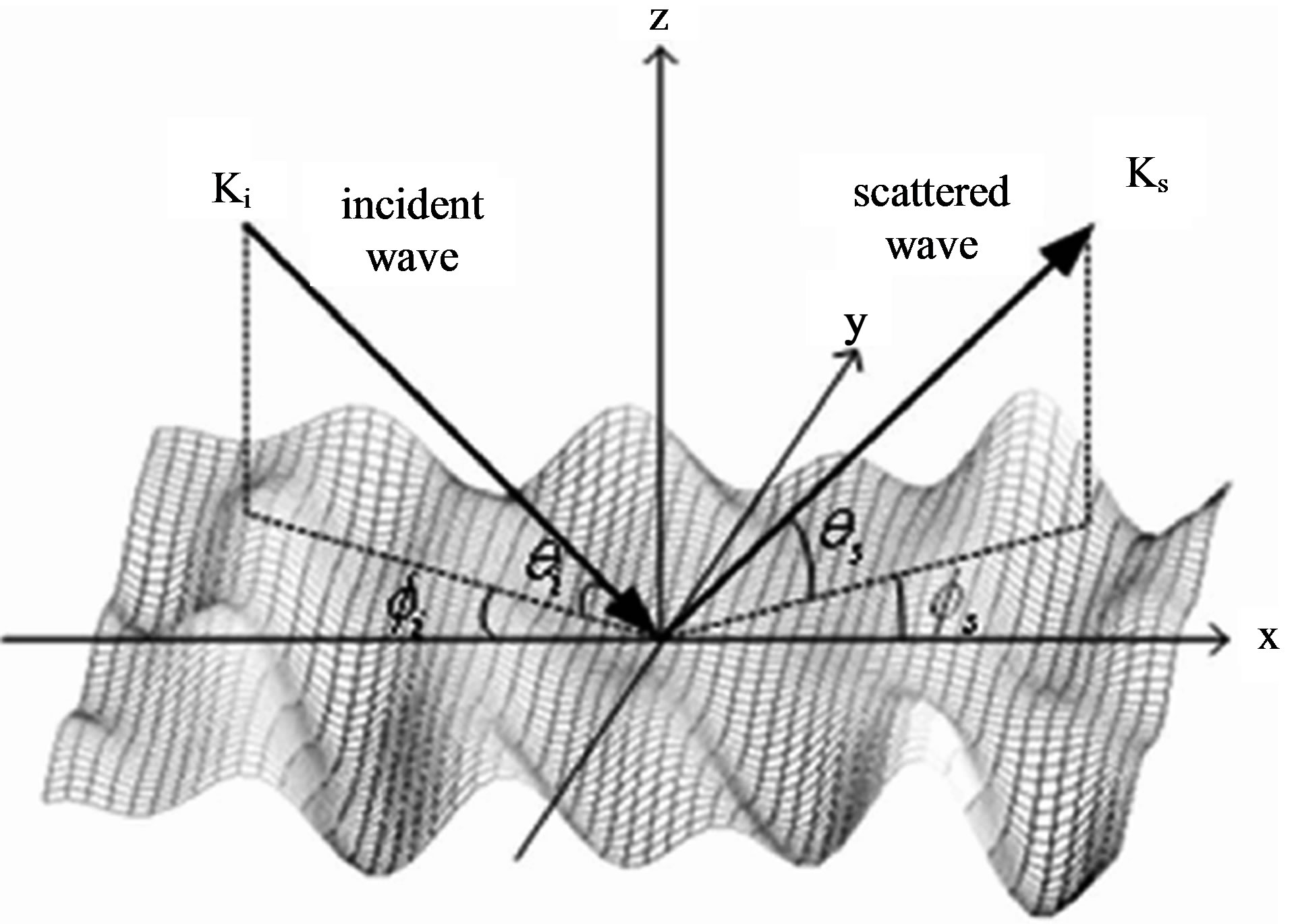
Figure 1. Configuration of the scattering problem with the incident wave vector , the scattered wave vector ks, the grazing incident angle θi, the azimuth incident angle
 , the grazing scattered angle θs and the azimuth scattered angle
 .
.
also taken into account and change with positive anticlockwise angles  in our simulations. The vertical component in the z-direction, kzi and kzsrespect
 . These terms are used to solve the scattering problem from a rough surface which statistical descriptions follow. Figure 2 shows examples of various angular configurations of interest for the different simulations presented in Section 3.
2.2. Modelling of the Isotropic and Anisotropic Surfaces via the Structure Function
The water and the seafloor are separated by a rough interface. In our context, this surface is considered plane on the average and is defined as
 (3)
(3)
where  is the position on the
  -plane, h is the deviation of the interface relative to its means plane
 , z is usually considered as a random process. To take into account the relief, its isotropic or anisotropic feature, when simulating scattering strength by a rough surface, the structure function is defined by Equation (4).
 (4)
(4)
where  and
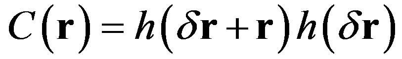
and  are respectively the height covariance at the position r and at zero lag. The two-dimensional covariance is defined as follows.
 (5)
(5)
with  the mean and
  the lag. One should notice that for a zero lag the autocorrelation is equal to 1 for
  divided by its variance.
One of the most typical isotropic structure functions is based on the grain sediment [9-12]. It is parameterized by a power-law spectrum and is defined by the following expression
 (6)
(6)
where r is the distance, w2 the spectral strength,  with
with  the spectral exponent
  is the gamma function. Nevertheless, to be able to change the roughness by modifying the correlation lengths, Lx and Ly respectively in the xand y-directions, and the rmsheight of the surface directly, two main structures functions are of interest in this study. One of the structure function, Dg is based on a Gaussian distribution. This type of distribution is well known when simulating scattering strength from a rough surface [6,8].
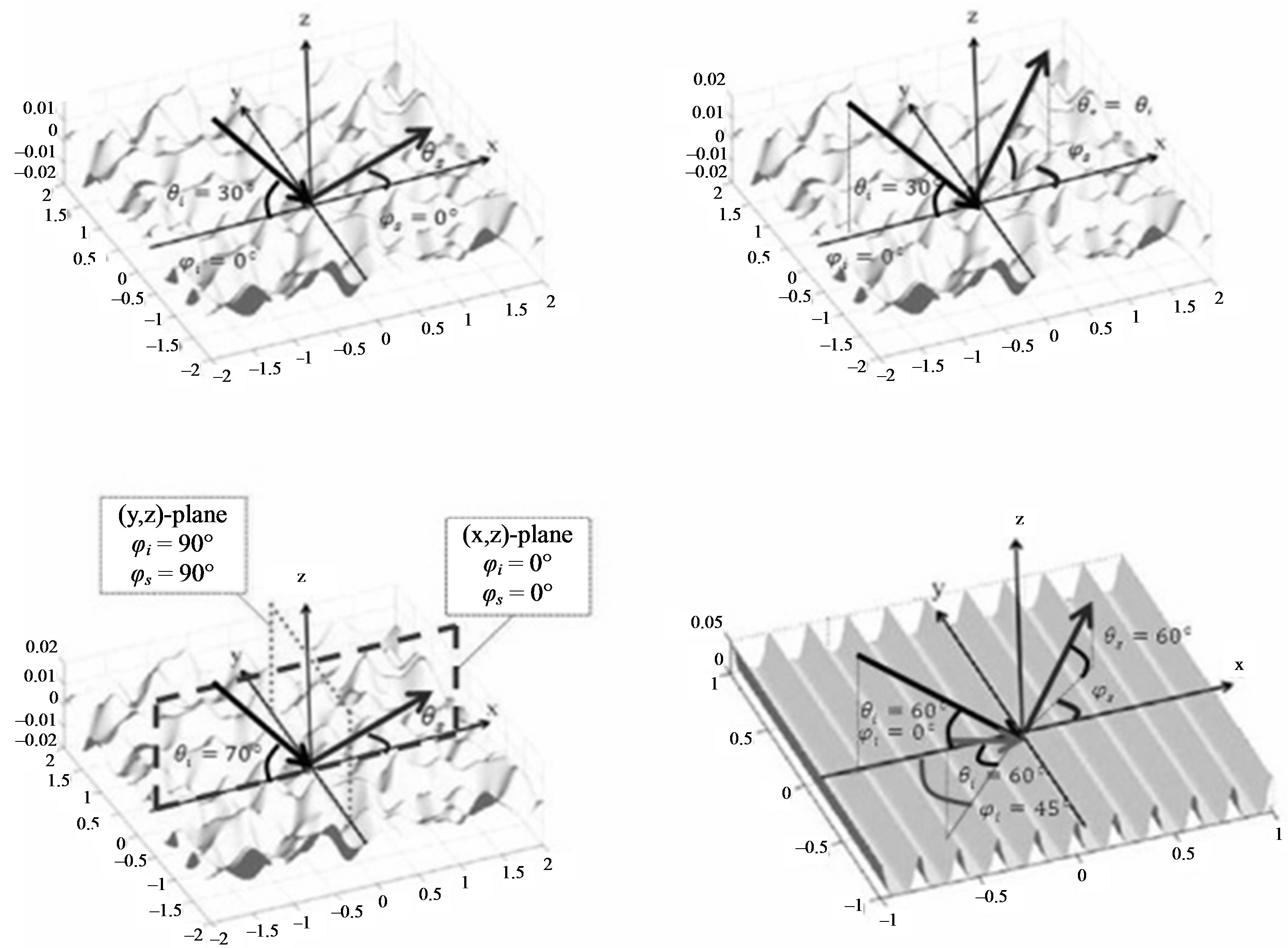
Figure 2. Angular configurations for different cases of interest: (top left) configuration for an isotropic surface as a function of the scattered angle ; (top right) configuration for an isotropic surface as a function of the scattered azimuth angle
 ; (bottom left) configuration for an isotropic surface as a function of the scattered angle
  into two different planes, the (x, z)-plane for
  and the (y, z)-plane for
 ; (bottom right) configuration for an anisotropic surface as a function of the scattered azimuth angle
  for different azimuth incident angle
 .
.
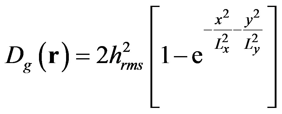 (7)
(7)
The structure function Dg is used either to model an isotropic surface or an anisotropic surface, depending on the values applied to the correlation lengths, Lx and Ly, respectively in the x and y directions. To deal with a part of periodicity and directionality of an interface, such as sandy ripples, we suggested another structure function, Dp which is based on a sine function.
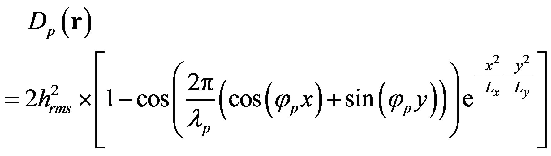 (8)
(8)
The structure function Dp is used to model a rough surface with periodic features, thus the surface is anisotropic and respect few statistical properties but mandatory such as the second-order stationary of the surface and that the surface is ergodic. In case of ripples, we assume that they do not change due to a particular event. Surfaces based on this structure function are in the following of this paper called ripples. The terms and
and are respectively the angle for the direction of the periodic sine shape and the wavelength of the sine function. The correlation lengths Lx and Ly allow to get a rough surface with periodic features more or less disordered.
Combining the three different structure functions allow us to simulate particular rough seafloors for predicting scattering strength.  is appropriate for a random rough surface made of a sediment which roughness properties have been estimated [10,12].
  is appropriate either for testing isotropic or anisotropic rough surfaces but without any feature about directionality or periodicity. Thus Dp which takes into account a quasiperiodic rough surface, is of interest since the effect on an acoustic wave is expected to be different from other types of anisotropic surfaces, and would give relevant information concerning the approach used to analyze the effect of sandy ripples.
To get one realization of a surface based on one of the previous structure functions, thus on one of the height covariances, first a Gaussian white surface is produced. Then its Fourier transform is weighted by the square root of the spectrum based on a chosen height covariance. Finally, the inverse Fourier transform gives one realization of the rough surface. The process to get a relief is summarized by Equation (9)
 (9)
(9)
where F is the Fourier transform, F–1 the inverse Fourier transform and B a Gaussian white noise. As an illustration, we present in the following three examples of rough surfaces.
Figure 3 shows one realization of an isotropic surface based on a Gaussian distribution which features are similar for all (x, y)-directions. Thus for such a surface, scattering model can be simplified from a two dimensional problem to one dimensional case.
Figure 4 shows one realization of an anisotropic surface based on a Gaussian distribution, but with different features depending on the direction. In the y-direction, the correlation length is longer, thus the surface has got a smoother shape compared to the x-direction where the correlation length is smaller.
Figure 5 shows one realization of an anisotropic surface based on the structure function . Other height fluctuations are observed. They are due to the exponential part of the structure function and they are related to the choice of very long correlation lengths versus
  in this case. The direction and the periodicity of the relief depend on
  and
and  respectively.
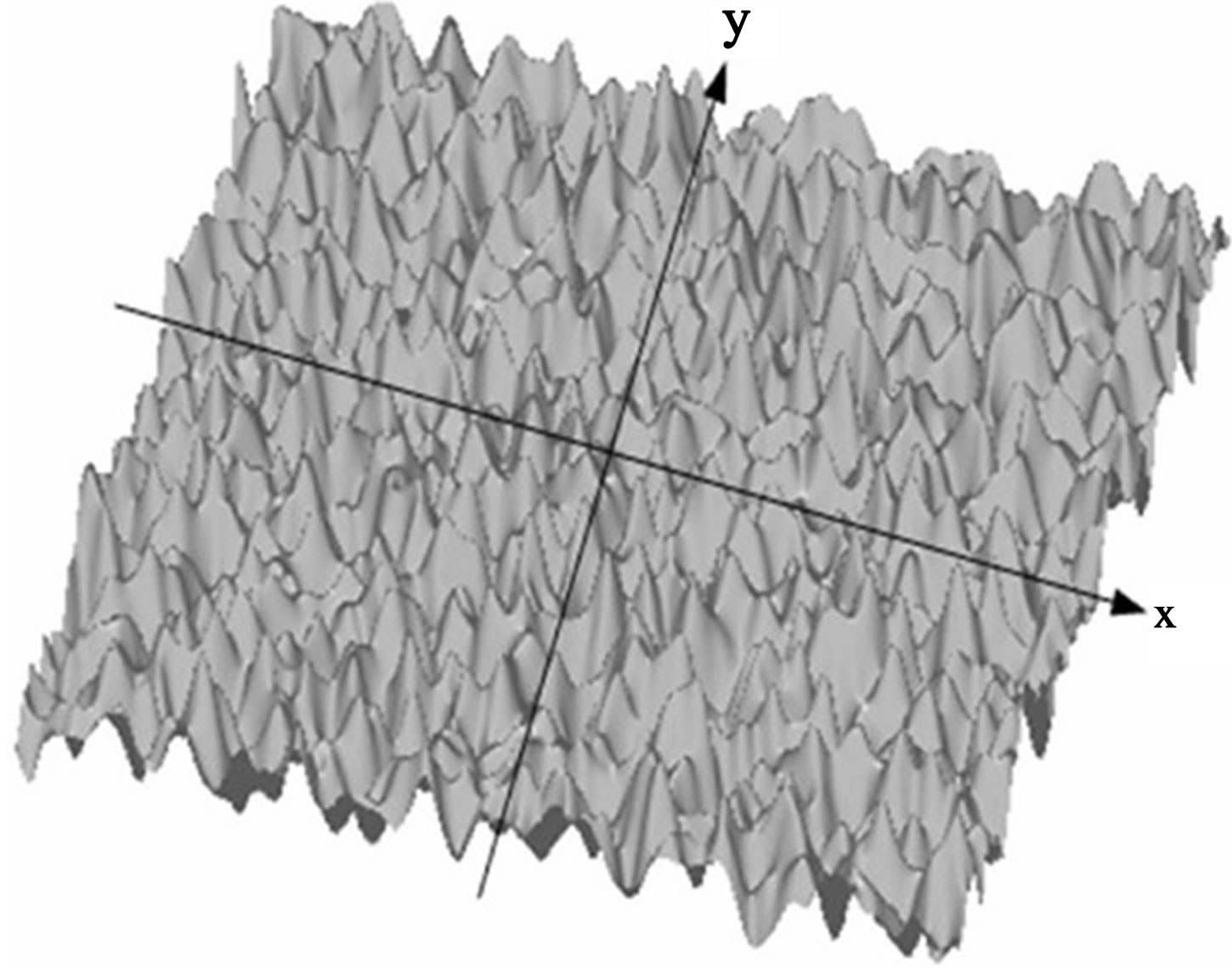
Figure 3. One realization of an isotropic surface, 5 m × 5 m, based on a Gaussian distribution (i.e. height covariance related to the structure function Dg(r)), with Lx = Ly = 20 cm, hrms = 5 cm.
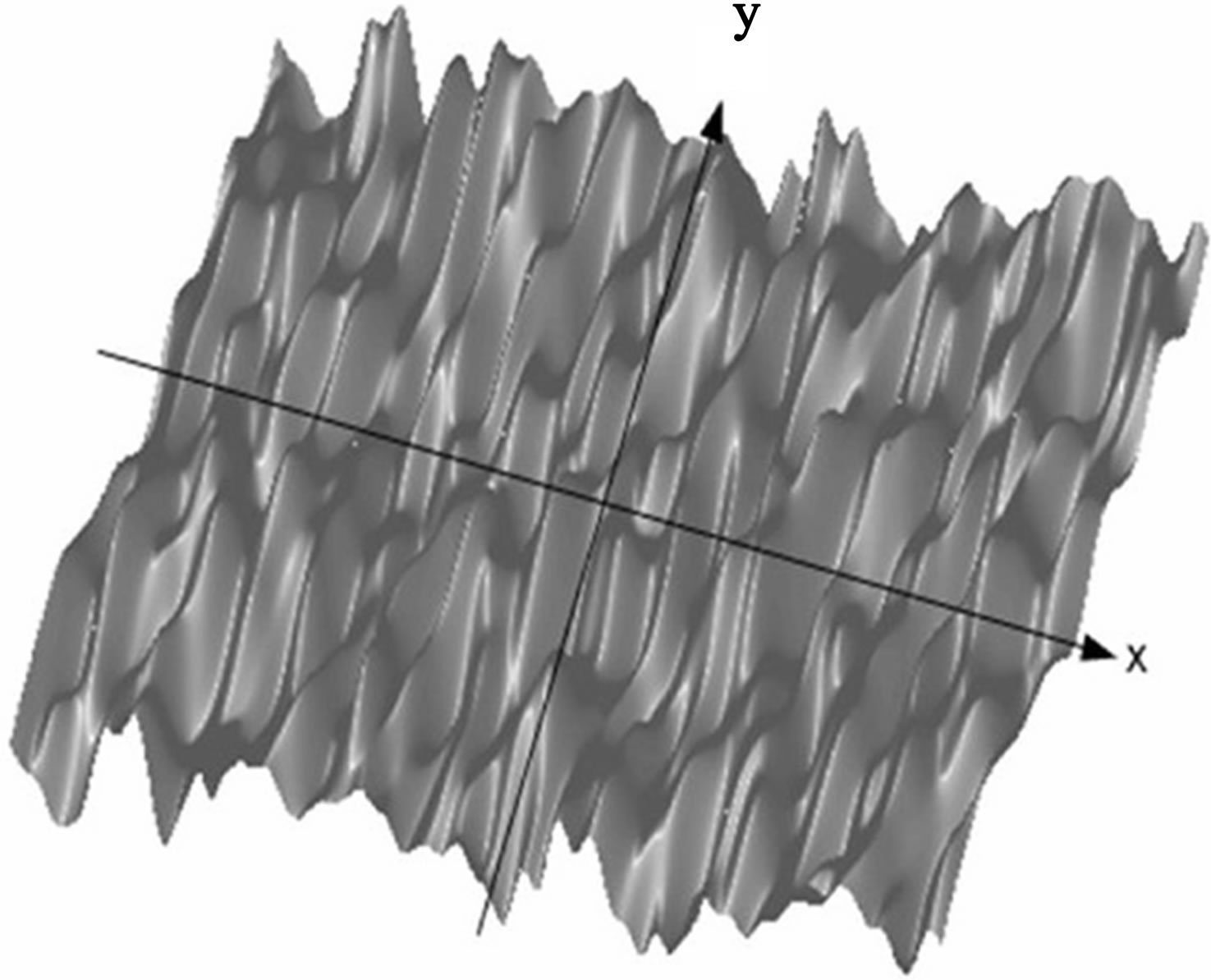
Figure 4. One realization of an anisotropic surface, 5 m × 5 m, based on a Gaussian distribution (i.e. height covariance related to the structure function Dg (r)), with Lx = 20 cm, Ly = 20 cm, hrms = 5 cm.

Figure 5. One realization of an anisotropic surface, 5 m × 5 m, based on a sine function (i.e. height covariance related to the structure function Dp(r)), with Lx = Ly = 300 cm, hrms = 5 cm, λp = 20 cm, φp = 30˚.
In the following simulations with such a type of relief, longer correlation lengths i.e.  will be used to get a large surface mostly dependent on the sine shape.
2.3. Modelling of Scattering Strength with SSA-1
The scattering problem is analyzed trough the scattering strength, SS, which is defined in decibel (dB) as:
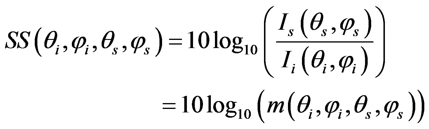 (10)
(10)
where  is the incident intensity,
  is the scattered intensity and m is the dimensionless scattering coefficient. The latter parameter represents how the acoustic wave is scattered from the rough surface (ref. at 1 m-distance over a 1 m2 surface). In this study, m is evaluated by using the first-order small slope approximation [12, 15,17,19] and is written as :
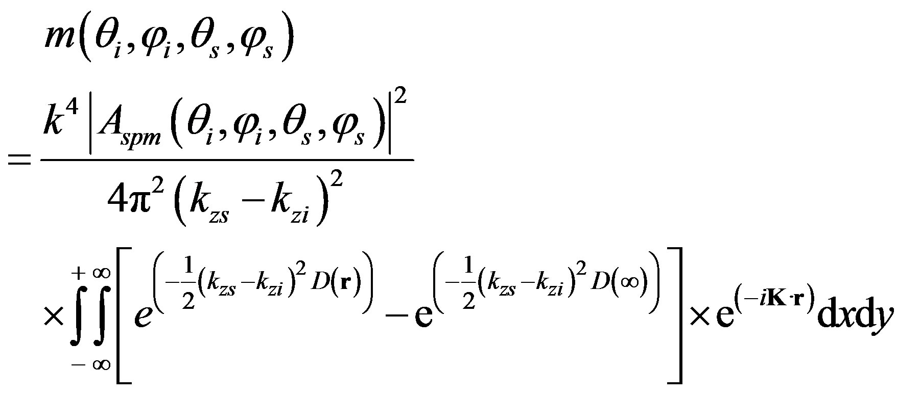 (11)
(11)
where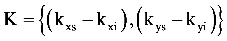 is the wavevector difference,
  is the position on the
  -plane and
  is the structure function defined in the previous section (see Equation (4)). In this study, scattering from sediment volume and multiple scattering are not considered, whereas losses of energy due to transmission into the sediment (from homogeneous or stratified seafloor) are considered through
 . Assuming that the sediment is fluid, this parameter depends on the plane wave reflection coefficients and on the incident and scattered waves as Equation (12) [12,22].
where  is the density ratio between sediment and water,
  is the wavenumber ratio between sediment and water, R is the plane-wave reflection coefficient depending either on the grazing incident angle
  or on the grazing scattered angle
 . One should note that the first-order small slope approximation coefficient could be shared into two major parts. Before the integral in Equation (11), sediment characteristics are defined, thus losses due to sediment are taken into account. Then the integral is related to the roughness of the seafloor which is the cause of the surface scattering phenomenon.
Concerning the choice of the roughness into the scattering model, our interest is to change easily the type of roughness when predicting scattering. The small slope approximation allows us to modify directly the height statistics, either by using true measurements of a rough surface or by using theoretical model to describe the approximation of first order is compared to a well-known bistatic method based on an isotropic surface, thus the effect of the isotropic roughness are shown. Then, SSA-1 is analyzed based on an anisotropic rough surface obtained by a Gaussian distribution. Finally, the model is used with another anisotropic roughness we suggested in
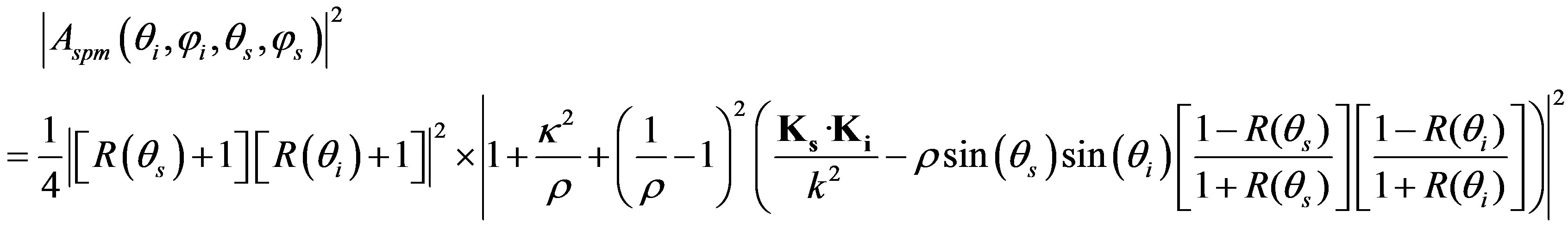 (12)
(12)
roughness. This modelling approach differs from many computations where anisotropy is directly implemented in the scattered field. The advantage of providing the roughness straightaway is also related to the unique limitation of SSA of first order: the elevation slopes have to be small enough. This is an asset compared to other scattering models where limitations are more numerous. To avoid shadow at very small grazing angles, higher orders of the SSA method could be considered [17,18]. Nevertheless the model of first order is relevant because the scattering coefficient is directly related to the roughness statistics and makes a roughness inversion process possible. In order to keep this ability and to take into account the limitation, the validity area compared to the type of roughness should always be kept in mind when analyzing the scattering data.
3. Simulations: A Parametric Study
This section is organized as follows: first the small slope this paper. The anisotropy of a rough surface is first examined, then the complexity of the anisotropic roughness is enhanced through the scattering strength obtained with SSA-1.
3.1. Study 1: Analysis of SSA-1 Compared to Jackson et al. Model (Case of Di(r))
The small slope approximation is used to predict roughness scattering from an isotropic surface based on the particular structure function  described by Equation (6) and always used in prediction by the bistatic model developed by Jackson et al. [11,12]. Both SSA and Jackson et al. models are first compared to analyzed the efficiency of SSA-1 assuming a basic environment made of sediment (fine sand or coarse sand) and based on an isotropic rough surface. Then scattering predictions are performed into different propagation planes, through a change of the scattered azimuth angle, to examine the properties of isotropy on scattering strength.
Two types of sediment, fine sand and coarse sand, are used as examples. The properties of these sediments are given in the following Table 1.
Figure 6 shows the prediction of the scattering strength, SS, as a function of the scattered angle  in one plane such as
 , for two kinds of sediments, fine sand (lines with circles) and coarse sand (line with squares). The predictions of the roughness scattering are made with SSA (dashed line with symbols) and compared to the bistatic model developed by Jackson et al. (full line with symbols) [11]. First of all, for two types of sediment and for the two different models, the scattering strength is higher in the specular direction for
  and decreases to a minimum value at grazing scattered angles. Then, apart from the specular direction and due to the particularity of each sediment (roughness dimensions
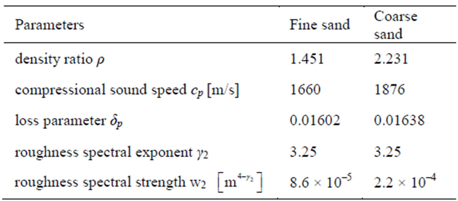
Table 1. Sediment parameters.

Figure 6. Predictions and comparisons (SSA-1 versus the bistatic Jackon’s model) of scattering strength, SS, as a function of the scattered angle θs for coarse sand (lines with squares) and for fine sand (lines with circles) for f = 30 kHz, θi = 30˚, φi = φs = 0˚.
and losses), the scattering strength is mainly higher for a coarse sand than for a fine sand. For both types of sediment, predictions are very close between SSA and the other bistatic model for most of the scattered angles. The small differences, about less than 2 dB, appear at particular scattered angles around  and around
  for these test cases. One should notice that the bistatic model developed by Jackson et al. is based on the interpolation of both the Kirchhoff approximation and the small perturbations method (KA being used in the specular direction and SPM in the other directions). The change from KA to SPM appear, in these simulated predicttions at scattered angles approximately around
  and around
 , which match the angles where differences were found. The small slope approximation being a unified method, small variations may be observed at the particular angles of interpolation of the other method.
Figure 7 shows the predictions of scattering strength as a function of azimuth angle  for the two types of sediments, between SSA and the other isotropic bistatic model, used in the previous test case. The incident and scattered angles are equal such as
 , with an azimuth incident angle set to
 . For both coarse
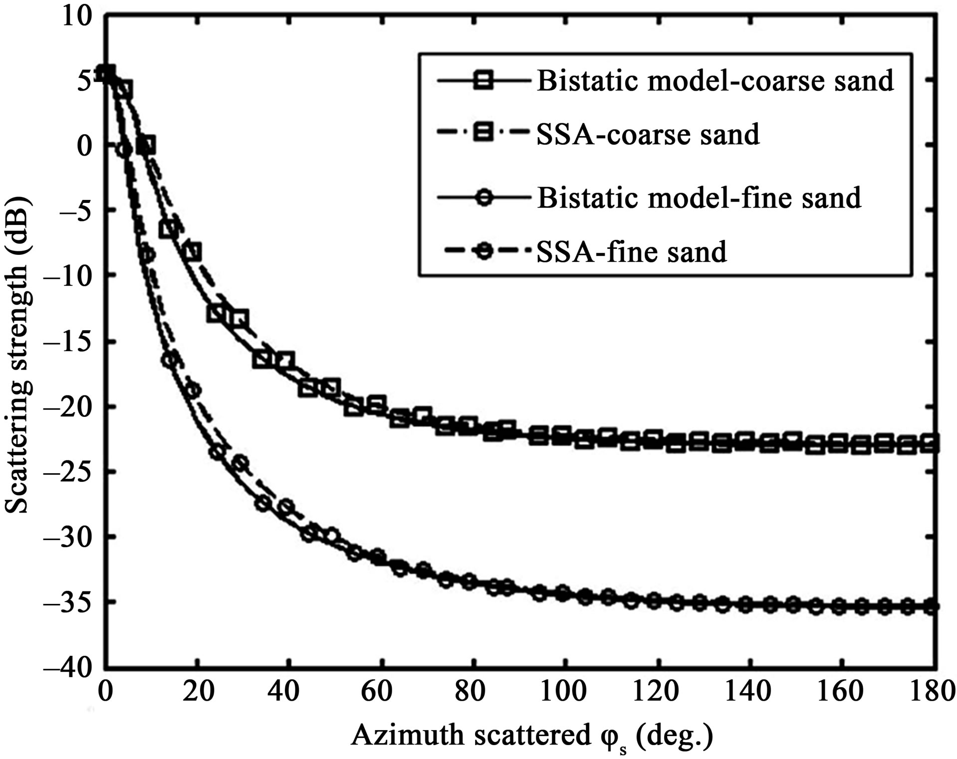
Figure 7. Predictions and comparisons (SSA-1 versus the bistatic Jackon’s model) of scattering strength, SS, as a function of the scattered azimuth angle φs for coarse sand (lines with squares) and for fine sand (lines with circles) for f = 30 kHz, θi = θs = 30˚, φi = 0˚.
sand and fine sand, and for the two different models, the scattering strength is higher at very low azimuth angles, with a maximum value for  which match with the specular direction. Then the scattering strength is mainly higher for a coarse sand than for a fine sand, particularly in a direction away from the specular direction and this feature has to be related to the roughness characteristics of each sediment (coarse sand rougher than fine sand) as well as to the losses parameters (fine sand attenuates acoustic waves more than coarse sand). For one given frequency, i.e. one given wavelength, the sediment made of fine sand is smoother than the coarse sand, thus the energy is spread in more directions for the coarse sand case. Finally, both predictions from SSA and predictions from the other bistatic model are very similar, especially at angles equal to the specular angle (around
 ) and at scattered azimuth angles higher than 60˚. Small differences, less than 2 dB, appear at azimuth scattered angles around
 . These angle area match the ones corresponding to the interpolation between KA and SPM.
Similarities of the simulations and very small differences of the same kind have been observed for other simulated cases where the type of sediment, or the frequency, and so on, were modified. Contrary to the bistatic model developed by Jackson et al., the small slope approximation is a unified method of the KA and SPM characteristics, that is why comparisons between SSA and the other bistatic model were first of interest. Then one advantage of the small slope approximation, through the expression given by Equation (11), is that different structure functions can be implemented directly with this model. Combine these primary results, based on an isotropic surface, allows to implement more complicated seafloors in the scattering process through the other structure functions  and
and .
.
3.2. Study 2: Analysis of SSA-1 with an Anisotropic Surface
3.2.1. Case of a 2-D Gaussian Structure Function Dg(r)
A Gaussian distribution through the structure function Dg is first used to model roughness (see the corresponding relief in Figure 4). The correlation length in the x-direction varied from the one in the y-direction such as  and
and . The variations of the height are taken into account in kh = 1.5 with k the wavenumber. For a fixed value of kh, kLx and kLy respect the limitation of SSA, that is assuming small surface slopes [18]. Figure 8 shows the prediction of the roughness scattering as a function of the scattered angle
 ,
,  , into two different planes, in the (x, z)-plane with
 , and in the (y, z)-plane with
  (see Figure 2 for the angular configurations of the planes). For predictions into the two different planes, the maximum value is obtained in the specular direction for
 . Then the scattering strength decreases to a minimum values obtained at grazing angles. In the (y, z)-plane of Figure 8, the scattering strength covers a narrow band around 70˚, such as an scattered angle area about 30˚ at –10 dB. In the (x, z)-plane, the energy is spread in more directions, such as the scattered angle area is equal to 80˚ at –10 dB. This phenomenon follows the expected behaviour: in the direction where the surface is smoother, the scattered energy is distributed around the specular direction whereas for rougher surfaces, the energy is spread in more directions.
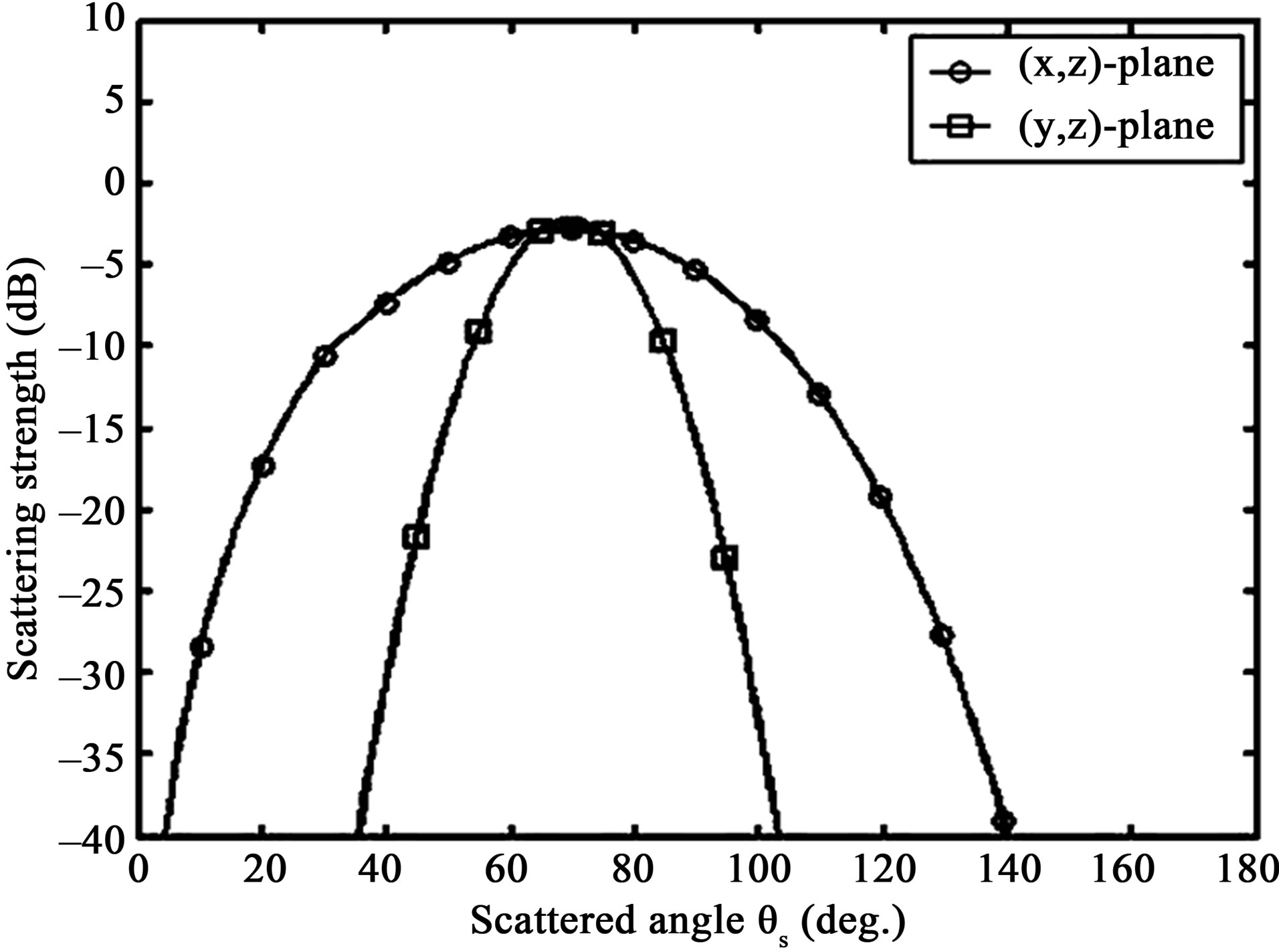
Figure 8. Prediction of scattering strength, SS, as a function of the scattered angle θs, for θi = 70˚; (line with circles) φi = φs = 0˚ thus for a plane where the correlation length is smaller kLx = 12; (line with squares) φi = φs = 90˚ thus for a plane where the correlation length is longer kLy = 20.
Figure 9 shows the scattering predictions, SS, as a function of the azimuth angle , and depend on
  and
and . Two simulations are compared. One is based on the anisotropic surface used previously which correlation lengths are
  and
and . The second simulation is based on an isotropic surface, such as correlation lengths are similar in both the x-direction and the y-direction, with
 . For the isotropic case, the maximum value is obtained in the specular direction for
  and decreases with higher values of
 . The scattering strength shows a minimum values for
 , thus in the backward direction. For the anisotropic case, the maximum value of the scattering strength is obtained in the specular direction for
 , then it decreases to a minimum around
  and finally increases in the backward direction for
 . Nevertheless, the value in the backward direction (–22 dB at
 ) is much lower than the value in the specular direction (about –5 dB fort
 ). The scattering strength is spread differently between simulations with an isotropic surface and with an anisotropic surface. The scattering strength is slightly higher in the specular direction, between
  and
and , of the anisotropic case, as well as for azimuth angles between
  and
and . On the contrary, between
  and
and , scattering strength from the anisotropic case is lower than from the isotropic case, with 10 dB difference at
 .
.
In the isotropic case, the scattering problem could be simplified to one direction which is not suitable in the anisotropic case since the entire surface induces an effect on the roughness scattering phenomenon.

Figure 9. Prediction of the scattering strength, SS, as a function of the scattered azimuth angle φs, with θi = θs = 70˚, φi = 0˚; (line with circles) different correlation lengths Lx ≠ Ly, (kLx = 12 and kLy = 20); (line with squares) Lx = Ly, (kLx = kLy = 12).
3.2.2. Case of a 2-D Quasi-Periodic Structure Function Dg(r)
The third type of structure function is now used for simulating the small slope approximation (see the corresponding relief in Figure 5) in the case of a quasi-perio dic relief such as a sandy bottom made of ripples. Scattering predictions are based on the structure function Dp defined by Equation (8), with a wavelength of , a rms height of 5 cm, a zero deviation angle of
  and large correlation lengths
 . The incident wave is defined by
  and a frequency of 50 kHz. Figure 10 shows predictions of the scattering strength as a function of the scattered angle
 . Scattering strength is given into two planes, in the (x, z)-plane (dashed line in Figure 10), with
 , and in the (y, z)-plane (line with squares in Figure 10) with
 . One should note that, in this test case, the (x, z)-plane in the transversal direction of the ripples (the acoustic waves propagate perpendicularly to the ripples directions) whereas the (y, z)-plane is in the longitudinal direction of the ripples (the acoustic waves propagate parallel to the ripples directions). Configurations of these propagation planes are depicted in Figure 2.
The scattering strength shown in Figure 10 and depending on the (y, z)-plane, is spread in a narrow band around 60˚ (about 5˚ at –10 dB), which is the specular direction. In this direction, the surface is much smoother and mainly depend on the correlation length . Such a scattering behaviour, most of the acoustic energy spread in the specular direction, is expected for a smooth surface. Then in the (x, z)-plane, the scattering strength varies strongly as a function of the scattered angle
 , with eleven maximum values around 10 dB down to –40 dB in this test case. The variation from one maximum
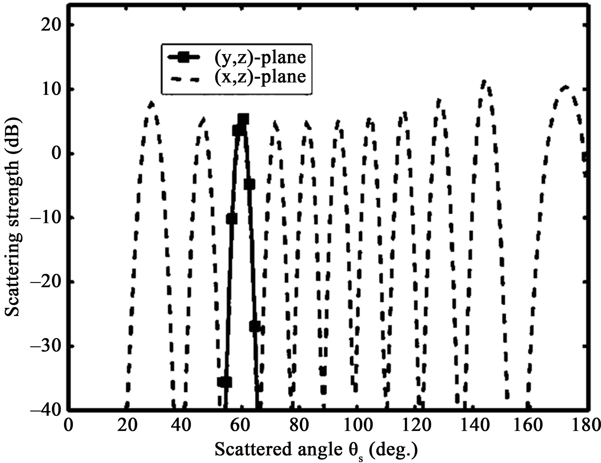
Figure 10. Prediction of the scattering strength, SS, as a function of the scattered angle θs, θi = 60˚; (dashed line) φi = φs = 0˚ thus propagation plane in the transversal direction to the ripples; (line with squares) φi = φs = 90˚ thus propagation plane in the longitudinal direction to the ripples.
value to one minimum one is very fast, about 5˚ of difference to go from one extreme value to the other. Furthermore, the angular lag between two maximum scattering strengths is approximately 10˚, particularly for scattered angles between  and
and . It increases a bit for scattering strengths obtained for
  and
and . These variations can be related to the shape of the roughness and thus through its structure function since the acoustics wavelength (3 cm for 50 Hz) is of order of the ripples dimensions (rms height of 5 cm and wavelength of 20 cm).
Figure 11 shows scattering strength, SS, as a function of the azimuth scattered angle  for three different azimuth incident angles
 ,
,  and
and . The incident and scattered angles are defined by θs =θi = 60˚ with a 50 kHz-frequency (see Figure 2 for the angular configuration). The rough surface is similar to the quasi-periodic sandy ripple relief used in the previous simulation, based on the structure function Dp defined by Equation (8), with a wavelength of
 , a rms height of 5 cm, a zero deviation angle of
  and large correlation lengths
 .
.
For , most of the energy is spread in the forward direction (around the specular direction for
 ) and in the backscattering direction (
 ). For an incident wave at
 , maxima are around
  and
and , which are respectively the forward and the backward directions. For
  a maximum strength appears at
  which is the forward direction, and also at 70˚ and 110˚. They correspond to positions of the scattered wave between the transversal and the longitudinal directions of the quasi-periodic relief. In this simulated case, the scattering strength is still higher if
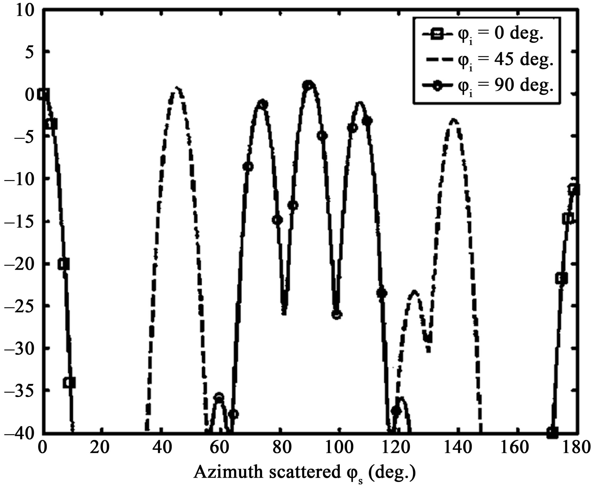
Figure 11. Prediction of the scattering strength, SS, as a function of the scattered azimuth angle φs, θs = θi = 60˚; (line with squares) φi = 0˚; (dashed line) φi = 45˚; (line with circles) φi = 90˚.
incident and scattered waves are in a same plane, the amount of energy spread in the backward direction is also important and scattering strength appear also in directions which are out from the forward and backward ones. Compared to the previous anisotropic case, the distribution of energy is different and is closely related to the structure function which has been modified from a Gaussian case to a quasi-periodic case. Thus directionality and periodicity of a seabed seem to be relevant on the scattering strength distribution.
4. Discussion
The first order small slope approximation is used to predict sound scattering by an anisotropic rough surface. With this model, we address the effects of seabed roughness with particular attention being given to simulation of the two-dimensional height structure function. The model is restricted by the usual small slopes assumptions, e.g., no sharp edges. The interest of this model is the possibility to change the roughness structure, either by using measured heights or theoretical heights. The replacement of such a surface by the one used in this study with a directional feature enhances the complexity of the numerical integral of SSA but expands the field of applications.
Predictions of the scattering strength from an anisotropic surface based on Gaussian distribution have shown that the choice of the positions of a source and a receiver compared to the rough isotropic surface is important and give different information. In a smoother direction of the surface, the scattering strength obtained considering one propagation plane would be spread around the specular direction. On the contrary, for a propagation plane placed in a rougher direction, the scattering strength is spread in more directions. For an anisotropic surface, the entire two-dimensionnal statistics of the surface should be kept instead of simplifying the model, to avoid inaccurate estimation of the scattering strength. Furthermore, assumeing an unknown surface, the differences obtained in the different propagation planes may be of interest for analyzing the seafloor from the scattering strength data. Then, combine results obtained from the anisotropic surface based on a quasi-periodic structure function, indicate as well the importance of taking into account the anisotropy in a model used for estimating the scattering energy distribution. The scattering strength is predicted differently from one propagation plane to another one. A seafloor with a particular anisotropic shape shows a scattering behaviour different from another particular anisotropic seafloor, i.e. a Gaussian distributed surface is different from a surface with a quasi-periodic shape and thus their statistics are dissimilar, that is why, in case of the ripple-shaped surface and for prediction as a function of the scattered angle, several values appear with approximately the same level and thus for different scattered angles. In this case, for a propagation plane in the transversal direction of the ripples, the specular direction is not the direction of interest. On the contrary, this direction is of importance for the simulations made in the propagation plane in the longitudinal direction of the quasi-periodic shape. Again, the results show the effect of choosing the position of the emitter and receiver compared to the roughness of the surface. Nevertheless, these very high-changing values, predicted by SSA-1 should be minimized in practice, since sonars or transducers depend on their own directivity, thus give an average value of the scattering strength.
Simulations and literature have shown the requirement of combining directionality of the anisotropy in the scattering model to correctly predict scattering strength in all directions. To better analyze these conclusions, tank experiments are required in order to model the appropriate structure function and validate the scattering process described in this paper, since data obtained from a controlled environment are always of interest to better understand a physical problem. It would be word worth also predicting roughness instead of roughness scattering via the structure function by extraction of this component.
5. Acknowledgements
This work was partly funded by the French Defence Procuration Agency (DGA) under research program ERATO (contract 09CR0001).
REFERENCES
- J. T. Anderson, D. Van Holliday, R. Kloser, D. G. Reid and Y. Simard, “Acoustic seabed classification: current practice and future directions,” ICES Journal of Marine Science, Vol. 65, No. 6, 2008, pp. 1004-1011. doi:10.1093/icesjms/fsn061
- A. J. Kenny, I. Cato, M. Desprez, G. Fader, R. T. E. Schüttenhelm and J. Side, “An overview of seabed-mapping technologies in the context of marine habitat classification,” ICES Journal of Marine Science, Vol. 60, No. 2, 2003, pp. 411-418. doi:10.1016/S1054-3139(03)00006-7
- K. Siemes, M. Snellen, D. G. Simons, J.-P. Hermand, M. Meyer and J.-C. Le Gac, “High frequency multibeam echosounder classification for rapid assessment,” Acoustics’08, Paris, 29 June-4 July 2008, pp. 4259-4264.
- L. Hellequin, J.-M. Boucher and X. Lurton, “Processing of high-frequency multibeam echo sounder data for seafloor characterization,” IEEE Journal of Oceanic Engineering, Vol. 28, No. 1, 2003, pp. 78-89. doi:10.1109/JOE.2002.808205
- C. Eckart, “The scattering of sound from the sea surface,” Journal of the Acoustical Society of America, Vol. 25, No. 3, 1953, pp. 566-570. doi:10.1121/1.1907123
- E. I. Thorsos, “The validity of Kirchhoff approximation for rough surface scattering using a Gaussian roughness spectrum,” Journal of the Acoustical Society of America, Vol. 83, No. 1, 1988, pp. 78-92. doi:10.1121/1.396188
- F. G. Bass and I. M. Fuks, “Wave scattering from statistically rough surfaces,” Pergamon Press, New York, 1979.
- E. I. Thorsos and D. R. Jackson, “The validity of perturbation approximation for rough surface scattering using a Gaussian roughness spectrum,” Journal of the Acoustical Society of America, Vol. 86, No. 1, 1989, pp. 261-277. doi:10.1121/1.398342
- D. R. Jackson, D. P. Winebrenner and A. Ishimaru, “Application of the composite roughness model to high-frequency bottom backscattering,” Journal of the Acoustical Society of America, Vol. 79, No. 5, 1986, pp. 1410-1422. doi:10.1121/1.393669
- D. R. Jackson, “APL-UW high-frequency ocean environmental acoustic model handbook,” Technical report, Seattle, 1994.
- K. W. Williams and D. R. Jackson, “Bistatic bottom scattering: model, experiments, and model/data comparison,” Journal of the Acoustical Society of America, Vol. 103, No. 1, 1998, pp. 169-181. doi:10.1121/1.421109
- D. R. Jackson and M. D. Richardson, “High Frequency Seafloor Acoustics, the Underwater Acoustics Series,” Springer, New York, 2007.
- J. W. Choi, J. Na and W. Seong, “240-kHz bistatic bottom scattering measurements in shallow water,” IEEE Journal of Oceanic Engineering, Vol. 26, No. 1, 2001, pp. 54-62. doi:10.1109/48.917926
- J. W. Choi, J. Na and K.-S. Yoon, “High-frequency bistatic seafloor scattering from sandy ripple bottom,” IEEE Journal of Oceanic Engineering, Vol. 28, No. 4, 2008,pp. 711-719. doi:10.1109/JOE.2003.819151
- A. G. Voronovich, “Wave scattering from rough surfaces,” Springer, New York, 1999.
- T. M. Elfouhaily and C.-A. Guerin, “A critical survey of approximate scattering theories from random rough surfaces,” Wave Random Complex Media, Vol. 14, No. 4, pp. 1-40, 2004. doi:10.1088/0959-7174/14/4/R01
- E. I. Thorsos and S. L. Broschat, “An investigation of the small slope approximation for scattering from rough surfaces. Part I. Theories,” Journal of the Acoustical Society of America, Vol. 97, No. 4, pp. 2082-2092, 1995. doi:10.1121/1.412001
- S. L. Broschat and E. I. Thorsos, “An investigation of the small slope approximation for scattering from rough surfaces. Part II. Numerical studies,” Journal of the Acoustical Society of America, Vol. 101, No. 5, 1996, pp. 2615- 2625. doi:10.1121/1.418502
- R. F. Gragg, D. Wurmser and R. C. Gauss, “Small slope scattering from rough elastic ocean floors: general theories and computational algorithm,” Journal of the Acoustical Society of America, Vol. 110, No. 6, 2001, pp. 2878-2901. doi:10.1121/1.1412444
- S. L. Broschat and E. I. Thorsos, “An investigation of the small slope approximation for scattering from rough surfaces. Part II. Numerical studies,” Journal of the Acoustical Society of America, Vol. 101, No. 5, 1996, pp. 2615- 2625. doi:10.1121/1.418502
- P. Traykovski, “Observations of wave orbital scale ripples and a nonequilibrium time-dependent model,” Journal of Geophysical Research, Vol. 120, 2007, pp. 1-19. doi:10.1029/2006JC003811
- J. E. Moe and D. R. Jackson, “First-order perturbation solution for rough surface scattering cross section including the effects of gradients,” Journal of the Acoustical Society of America, Vol. 96, No. 3, 1994, pp. 1748-1754. doi:10.1121/1.410253