World Journal of Engineering and Technology
Vol.03 No.01(2015), Article ID:53751,13 pages
10.4236/wjet.2015.31001
Using Neural Networks for Simulating and Predicting Core-End Temperatures in Electrical Generators: Power Uprate Application
Carlos J. Gavilán Moreno
Cofrentes Nuclear Power Plant, Iberdrola Generación Nuclear, Valencia, Spain
Email: cgavilan@iberdrola.es
Copyright © 2015 by author and Scientific Research Publishing Inc.
This work is licensed under the Creative Commons Attribution International License (CC BY).
http://creativecommons.org/licenses/by/4.0/


Received 13 January 2015; accepted 30 January 2015; published 3 February 2015
ABSTRACT
Power uprates pose a threat to electrical generators due to possible parasite effects that can develop potential failure sources with catastrophic consequences in most cases. In that sense, it is important to pay close attention to overheating, which results from excessive system losses and cooling system inefficiency. The end region of a stator is the most sensitive part to overheating. The calculation of magnetic fields, the evaluation of eddy-current losses and the determination of loss-derived temperature increases, are challenging problems requiring the use of simulation methods. The most usual methodology is the finite element method, or linear regression. In order to address this methodology, a calculation method was developed to determine temperature increases in the last stator package. The mathematical model developed was based on an artificial intelligence technique, more specifically neural networks. The model was successfully applied to estimate temperatures associated to 108% power and used to extrapolate temperature values for a power uprate to 113.48%. This last scenario was also useful to test extrapolation accuracy. The method is applied to determine core-end temperature when power is uprated to 117.78%. At that point, the temperature value will be compared to with the values obtained using finite elements method and multivariate regression.
Keywords:
Neural Network, Error, Temperature, Core-End, Generator, Power Uprate

1. Introduction
In the power generation industry, there is a question with no consistent answer over time: should we invest in new generation assets and increase installed power? Or on the contrary, should we improve existing installations to increase their performance and therefore their power output as well?
In economic scenarios such as the current one, in which power demand is stagnated and the expansion policies of most Western Europe utilities are a thing of the past, the question answered is the second one, relating to increased performance and power output of existing generation assets. By choosing the second option, investment is minimized and production unit costs optimized because, although actual production expenditure remains stable, energy generation increases.
For all these reasons, many authors develop solutions based on power uprates or comprehensive performance enhancements [1] . The solution presented in this paper involves a power uprate applied to a synchronous generator, which considering that voltage is constant and increased intensity through stator coils. Without getting into the peculiarities of steam generation process limitations or combustion improvements, this type of solutions has a common bottleneck: the thermal capacity and margin of generator winding insulation. In terms of power uprate, these essential parameters are constraining because an increase of associated intensity results in higher generator conductor temperature, especially in the critical area known as end-core. That is the reason why it is vital to determine expected temperatures in these generator areas beforehand, as actual temperature values will condition the feasibility of power uprate and additional power. In other words, this determination will ultimately impact power uprate viability.
After determining end-core temperature as a limiting parameter [2] , it is time to perform calculations and extrapolations aimed at verifying if final extrapolated or calculated temperature is in fact below the acceptance criterion, which in this case will be the type B insulation limit (130˚C) [3] -[7] .
Currently, there are two types of techniques to estimate end-core temperature: the finite element method (FEM) [8] and the regression estimation method [9] . The first method (FEM) is numerical, complex, more precise, resource intensive and requires an accurate internal generator geometry knowledge, which means that it is usually limited to OEMs or costly reverse engineering processes. Mathematically speaking, the second method is simpler and more accessible, but it renders more inaccurate results since the simulated process is significantly non-linear. The method proposed here is based on artificial neural networks because of their predictability, universal prediction, reality-adapted results, accessibility and easy implementation. The main challenge of this method is the need to have operational data from the machine under analysis so as to learn and create a reliable database from which to extrapolate power uprate results. Out of all neural networks, Feedforward architecture is chosen as it adapts to the purpose of adjusting and extrapolating.
Using the abovementioned neural network requires a training process based on actual machine conditions and data, which means that it is necessary to have information on known operating states. Once the network simulates end-core temperatures with a minimum error under known conditions, it is time to extrapolate temperature values under power uprate conditions. In this case, there are available data for generator and end-core temperatures for an initial rated generator power of up to 108.57%. These data will be used to train the network and extrapolate end-core temperature values for power levels of up to 113.48%. Once this power is reached, the accuracy of the first extrapolation value will be checked. If extrapolation is accurate, the network will be rendered adequate and data will be gathered for a 113.48% power level which, together with available 108.57% power values, will be used to train the network and extrapolate data for a power level of 117.78%, which is what the licensee actually wants. The extrapolated value will be compared to the results obtained using the abovementioned two methods so as to analyze numerical values, calculation capabilities and method advantages.
2. Case Description and Methodology
The problem described will be analyzed in an energy production plant with the aim of determining the expected electrical generator core-end temperature for a power uprate.
The model is developed to estimate, simulate or extrapolate the core-end temperature in a liquid and gas cooled 4-pole [10] [11] , electrical generator once the power uprate is finalized. That is the simulation should provide the expected temperature under conditions in which the generator has never operated or being tested. The ultimate reason for this simulation and its results is to verify that type B insulation limits are not exceeded. An example of this type of generators is seen in Figure 1.

Figure 1. Modeled generator layout.
After defining the problem and determining the equipment (generator) on which power uprate simulations and forecasts will be carried out, it is time to establish the physical model so that target parameters can be known, calculated and extrapolated.
Inside the generator there are several physical phenomena: electrical, magnetic, thermal and fluid-mechanical. The phenomenon favoring energy creation inside the generator is the rotation of the magnetic field, which is in turn caused by the electrical phenomenon of rotor turning and subjected to intensity. In this case study, turning speed is considered to be constant. A secondary phenomenon is stator electricity, characterized mostly by phase (3) intensity and terminal voltage. These two phenomena are responsible, together with grid conditions (reactive power), for heat and thermal generation due to parasite processes and losses.
Inside the water-and hydrogen-cooled generator there are two heat sinks: one for water and the other for hydrogen. The variables regulating the hydrogen heat sink are hydrogen purity and pressure as they impact the thermal coefficient of the gas, the thermal difference of hydrogen inside the coolers and also hydrogen temperature at the cooler outlet. In the case of coil water, the key variables are coil water flow rate and water temperature in generator inlet and outlet.
These variables, which can be seen in Table 1, will be used to develop the model. These parameters will be neural network inputs.
The critical part in this type of generators is the core-end, which is exposed to magnetic flux and significant eddy current-induced losses in the tooth tips of the first magnetic plate packs. In this location the cooling effect of the hydrogen and water is not fully developed so the temperature is always higher than any other location. Output variables will be the core-end tooth tip. Table 2 shows the name and location of thermocouples installed in these unfavorable locations.
For the purposes of this study, an artificial neural network has been selected as the best method because it is a general tool [12] and therefore works well for both lineal and non-lineal phenomena, hence covering a wide range of possibilities. It is important to take into consideration that the neural network is a universal approximator [13] [14] allowing for generalization and extrapolation [15] .
Once the conceptual model, tool and calculation process input and output variables have been determined, it is time to present the model scheme in which calculation stages, acceptance criteria values and admissible error rates will be developed. Figure 2 shows a graphic representation of this process.
The process starts by measuring the value of variables in Table 1 and Table 2 under operating conditions in which generator power is below 108.57%. These data are used to test the network based on the following criterion: variable values in Table 1 should allow the network to generate Table 2 values which should be compared to real values to ensure a maximum difference of 0.1˚C. This neural network is used to extrapolate end-core temperature values (Table 2) for a power level of 113.48% of initial rated generator power. Extrapolated values are compared to those obtained when the plant reaches the specific power level. If extrapolation values have a difference of less than 5% compared to plant-measured values, the network is rendered adequate and can be used

Table 1. Independent variables.
Table 2. Model output variables.
for final extrapolation.
As previously mentioned, the power uprate value targeted by the licensee is 117.78%, for an apparent power of 1277 MVA and a power factor of 0.95. For end-core temperature value extrapolation, a network entry data sheet needs to be put together, similar to Table 1. Values should include measurements of up to 108.57% plus those measured at the 113.48% stage of initial rated power. The same variables (Table 2) measured under the same conditions, are used to establish network training parameters.
In parallel, the values of Table 1 variables are established, as determined by design, for an extended power level of 117.78% (represented in Table 3).
Given extrapolation criticality and the stochastic nature of neural networks, this final step will be described in further detail. The neural network will be tested using known data (108.57% and 113.48%). When the point in which the calculated error of end-core temperature values is lower than 0.1˚C, temperature values are calculated in the same point for a power level of 117.78%. In this case, the input variables included in Table 3 will be used as input neural network data. This process will be repeated 30 times, which means that for every point of interest (Table 2), 30 temperature values will be obtained. The expected value will be the average of all of them in each point of interest; temperature values will be determined for a confidence interval of 95%.
3. Model Definition
The method based on artificial neural networks provides a solution of acceptable quality with very little effort.

Figure 2. Flow schematic of the temperature determination process at 117.78% power.
Table 3. Variables and values used in the extrapolation to 117.78%.
A multilayer neural network (Feedforward) has a feature that was mentioned before: it is a universal approximator. The neural network is conditioned by the input layer, the output layer, as well as the transfer functions that together with the synaptic weights and biases, make up network parameters. Figure 3 shows a proposed network layout.
Focusing on the problem under analysis, a multilayer Feedforward network will be adopted. The neural network will have three layers: input, output and hidden. The first layer (input) will have as many neurons as variables in Table 1 [15] . The output layer will have six neurons, one for each output variable included in Table 2. The design of the hidden layer is critical to convergence, error evolution and training performance [16] [17] . The number of neurons in the hidden layer will be selected as follows:
・ The number of hidden neurons should be in the range between the size of the input layer and the size of the output layer. So the range will be between 15 and 6.
・ The number of hidden neurons should be 2/3 of the input layer size, plus the size of the output layer. In this particular case they are 16.
・ The number of hidden neurons should be less than twice the input layer size, so the number should be less than 12.
Obviously only the second condition is not coherent with the first and third, therefore, it will be neglected. So finally 12 neurons will be implemented in the hidden layer (see Figure 4).

Figure 3. Typical layout of a Feedforward-type neural network.

Figure 4. Neural network architecture for this model.
3.1. Training
Once the architecture to be used in a particular problem has been defined, it is necessary to adjust the neural network weight through the training process. The training process is composed of three sub-processes: learning, validation and test. The learning algorithm includes a problem of inference associated to free network parameters and related neuron connections.
The learning process of a Feedforward neural network is ought to be supervised because network parameters, known as weights and biases, are estimates based on a set of training patterns (including input and output patterns). In order to estimate network parameters, a backpropagation algorithm is used as generalization of the delta rule proposed by Widrow-Hoff [13] [14] . Learning implies weight adjustment by comparing the neural network output to measured value, to minimize error. The error will be calculated as the mean squared error between the simulated temperature and the real (measured) temperature.
Figure 5 shows a detailed training process including three clearly differentiated phases. The first phase is learning as such. In this phase, weights and biases characterizing neurons and their connections are determined by means of the learning process described above. In this phase, 90% of available data is used. After training, it is necessary to determine the error made when comparing network output to actual data and if error is lower than a specific value (0.1˚C in this case), the next phase can be initiated. The second phase is validation. In this phase, output values are calculated using 5% of available data not used during the training phase. If error is less than 0.1, a test is performed and the network rendered “trained”; if the error is not less than 0.1˚C, the learning phase must be repeated until the validation error value meets the target.
Figure 6 shows the evolution of the learning error, validation and test.
This error estimates how the neural network can be adapted to the problem under analysis. Process results include not only error evolution during the learning phase, but also error distribution throughout the different phases as well as fitting between network-simulated values and real values. These results are specifically addressed in the following section.

Figure 5. Training flow diagram.
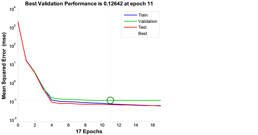
Figure 6. Error evolution during the training, validation and test phases.
3.2. Error Evaluation
This section will address network errors, both in the training and validation phases. The analysis will be more thorough than a mere evaluation of Figure 7, focusing on aspects such as error biases, error morphology, error evaluation and inter-phase error adjustment. Figure 7 and Figure 8 illustrate the analysis.
The first analyzed figure (Figure 7) is a histogram of error values that are associated to the learning, validation and test phases. The figure shows the error probability function as normal distribution, with an average near zero and a very small variance (<0.1˚C). As a result, it is considered white noise, being very consistent, structureless and not causing any bias.
In order to support the previous analysis, a linear regression between the data obtained by the trained neural network and the data actually measured (Figure 8), was conducted. This comparison was made in four different scenarios: the last learning, the last validation, the test and finally, a joint analysis. This analysis results in three important parameters related to one another and to the previously presented concept of normal probability function error. The three parameters are: R or correlation coefficient, slope of the regression line and the value of output data when the target data is zero.
・ R values or correlation coefficient are near 1; this means that neural network temperature output values match real values. It is also worth mentioning that data dispersion near the line is very small or null.
・ Line slope values are 1 in all cases, meaning that simulated values and measured values have a 1:1 equivalence. The result obtained is very close to reality, with an average error value of zero.
・ The simulation is slightly biased (value lower than 0.1), but it is considered residual and therefore negligible. The former analysis concludes that simulated values are realistic, with a high degree of accuracy.
4. Simulation Results
In the previous section, the neural network was dimensioned and trained, and errors and results were analyzed in scenarios in which the temperature value provided by the trained neural network was taken as real.
According to the scheme in Figure 2, the next step is the simulation or extrapolation of end-core temperature values for operating conditions of up to 113.85% of the original rated power. The full set for this extrapolation (simulation) is comprised of 145 sets of variables (Table 1), which means the network will provide 145 sets of 6 different temperatures, as described in Table 2.
In parallel and considering that this operational condition is feasible for the plant, real temperature measurements are taken at the selected points (Table 2).
Measured points are compared to extrapolated (simulated) data by means of four graphs or techniques:

Figure 7. Error histogram.

Figure 8. Training phase distribution and goodness of fit.
correlation, histogram, error-active power correlation and temperature versus time plot for extrapolated (simulated) and measured cases.
An analysis of linear correlation between extrapolated (simulated) and measured temperature data leads to the conclusion that the simulation is good when the adjustment value obtained is 0.94092 (Figure 9).
A histogram analysis (Figure 10) reveals that in absolute terms, error has an average value of 0.4082˚C. Furthermore, the negative sign indicates that extrapolation (simulation) provides results exceeding average machine values, indication that gets confirmed after observing in Figure 9 that, for the most part, points are above the y = x equation line. This fact supports the purpose of this work as it provides extrapolated (simulated) values with a slight safety margin.
According to Figure 10, the extrapolation error is a normal probability function, with an average of −0.4082˚C (negative) and a standard deviation of 0.2984. The absolute error value represents an error of 0.68% above the real value. The 95% error confidence interval is between −1.005˚C and 0.1886˚C. The error is lower than 5%, so the extrapolation is considered to be valid.

Figure 9. Correlation between real values and simulated values.
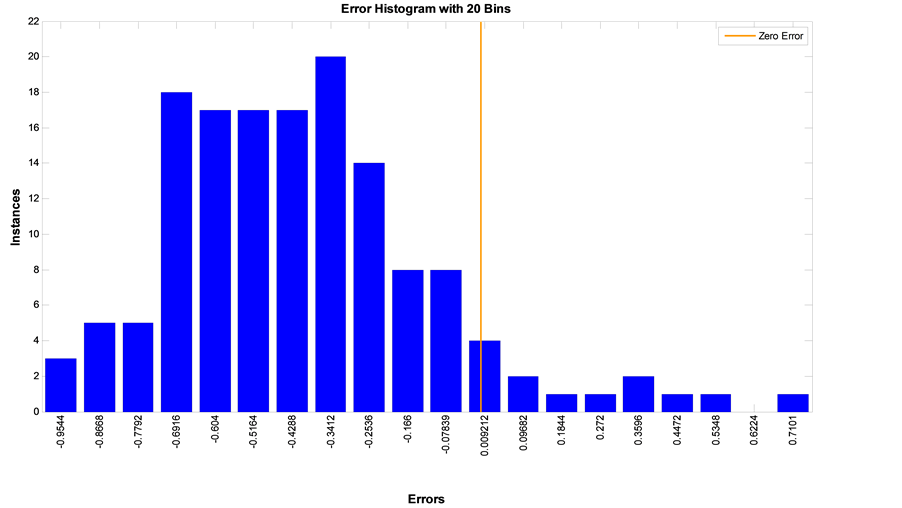
Figure 10. Histogram of errors made during the extrapolation.
An analysis of active power and error correlation (Figure 11) leads to the conclusion that there are no clusters. It is also noted that as power increases, error reduces. This behavior is coherent with the information in Figure 9, which shows that a temperature increase (real and simulated) shortens the gap between both temperature values (eventually tending to zero). As a result to temperature increases, the points in Figure 9 tend to be above the y = x line.
Finally and for information purposes, Figure 12 shows the time evolution of extrapolated (simulated) and measured machine temperatures, noting that they are well adjusted and look similar. It is also confirmed that simulated or extrapolated values are slightly higher than measured values.
In summary, it was verified that during the training phase, error is lower than 0.1˚C whereas in the extrapolation

Figure 11. Error vs. active power (MWe).

Figure 12. Extrapolation in the time domain.
phase for values at a power level 113.85%, error is under 5%. Thus, it is concluded that the neural network simulates well the thermal status of the generator and its core-end. The data and analyses provided in previous paragraphs support the credibility and robustness of the method, which is ultimately aimed at determining core- end temperature in advance, for a 117.78% power level in relation to initial generator rated power.
This is a clear, extreme case of extrapolation, which as opposed to a 113.85% power level (in relation to initial rated power), will render values that cannot be checked. That is precisely the motive for this work: obtaining an estimate to make decisions on the viability of a power uprate. In this case other simulated values are available. For this additional simulation, the finite element method (FEM) and regression method have been used.
As established in the introduction and the sequence of Figure 2, the network will be retrained using initial data for a power level of 108.57%, before increasing those values based on measured data for a power level of 113.85%. This will render a trained network with an error nearing zero in the training phase, as seen in Figure 13, which also shows that the error confidence interval at 95% is ±1.00˚C.
In order to be coherent with previous analyses, correlations between real measures and neural network results during the training, validation and testing phases are shown in Figure 14. The correlations included in Figure 14 have correlation index values of 0.999, (i.e., very near to 1), which indicates highly accurate linear adjustment between simulated and real values, indication confirmed by the fact that all points in the correlation graphs are on the y = x equation line. With regards to the bias, the regression line intercept is considered to be 0.066˚C, a negligible value leading to the conclusion that network-simulated values are equal to real values.
Once the network is trained and due to the stochastic nature of neural networks, the training-simulation process should be repeated at least 30 times. In other words, it is important to train the network before applying the entry values of variables included in Table 3. One measurement point, thermocouple Tc82, has an average temperature of 87˚C with a standard deviation of 3.15˚C. In light of this, expected thermocouple temperature for a power uprate condition (117.78%) will range between 93.30˚C and 80.70˚C, with a probability of 95%.
Comparison with the values of other evaluation methods is shown in Table 4.
The values of Table 4 allow us to conclude that finite element method values and neural network results are consistent, with similar magnitudes and values. Going a step further, it is possible to state that the temperature value obtained with the FEM is covered by the statistical result of the neural network. As for the extrapolation method, values are high and near the limit, although below the acceptability criterion for type-B insulation.
Considering all these information and findings, it is possible to assert that the required power increase is viable without the need to modify any auxiliary generator parameter.

Figure 13. Error histogram during the second training sequence.

Figure 14. Value adjustment and correlation with measured values.
Table 4. Values simulated by the neural network and other systems for the worst case.
5. Conclusions
This study leads to many conclusions. Firstly, the neural network used is found to be not only a good simulator of the core-end temperature value in an electrical generator, but also a valid option to predict and determine the expected power uprate core end temperatures. This concept can be broadened by using the network to determine core-end temperatures for non-tested conditions, hence considering this a forecasting model.
After looking at the three models used (Table 4), a study and analysis strategy can be established. When the dataset is scarce, the expected temperature can be determined using a multivariate regression model. If it is determined that the expected temperature is lower than the specification for a type B insulation, the process can move forward. In the next step, it is necessary to gather generator data using a monitoring system and to develop the neural network so that thermal generator behavior can be modeled for a wide spectrum of operational conditions. In this case, it is also possible to extrapolate core-end temperatures for power uprate conditions. If it is verified that the expected temperature is still below the type B insulation criterion, then a finite element model can be developed when the value is very near to the limit or very far from the upper limit. This strategy ensures reliability while minimizing costs and risk levels.
This tool allows a sensitivity study to determine the effect of each of the 15 input variables on the final result, hence favoring the establishment of cooling strategies if needed and anticipating unexpected scenarios and the best way to respond to them. This model is a very useful generator simulator, improving decision-making pro- cesses and training strategies for power plant operators.
Finally some remarks about the performance of the simulated electrical generator should be highlighted. The simulated electrical generator has an apparent power of 1120 MVA, and is working at a point of 0.98 power factor. In situations in which the grid has a capacitive behavior, the operator must reduce active power to avoid unwanted situations or cross the URAL curve (limit). This power reduction constitutes an economic impact. The proposed power uprate, in addition to setting the thermal behavior of the magnetic core, and new URAL curve based on that, leads to optimize the operation of the generator and the benefits of its exploitation. The other important point is that no plant modifications are required for the power uprate because none auxiliary system is limiting.
References
- Katayama, H., Takahasi, S., Nakamura, H., Shimada, H., Ito, H., Coetezee, G.J. and Claassens, F.A. (2006) A Successful Retrofit of Old Turbo-Generators Having Various Technical Problems. CIGRE. Ref. A1-206.
- Gunar, K. (2008) Stator Core-End Region Heating of Air Cooled Turbine Generators. Ed. VDM.
- IEC 60085-1 (2007) Thermal Evaluation and Classification of Electrical Insulation.
- IEEE Std 56 (1977) IEEE Guide for Insulation Maintenance of Large Alternating-Current Rotating Machinery (10,000 kVA and Larger).
- IEEE Std 95 (1977) IEEE Recommended Practice for Insulation Testing of Large AC Rotating Machinery with High Direct Voltage.
- IEEE Std 433 (1974) IEEE Recommended Practice for Insulation Testing of Large AC Rotating Machinery with High Voltage at Very Low Frequency.
- IEEE Std 434 (1973) IEEE Guide for Functional Evaluation of Insulation Systems for Large High-Voltage Machines.
- Lu, D.Q., Huang, X.L. and Hu, M.Q. (2001) Using Finite Element Method to Calculate 3D Thermal Distribution in the End Region of Turbo Generator. Proceedings of the CSEE, 21, 82-85.
- Li, J.Q., Li, H.M. and Lu, Z.P. (2003) Research on Temperature Rise of Stator Iron-Core End Region of Turbine Generator. The 5th International Conference on Power Electronics and Drive Systems, 1, 766-770.
- Klempner, G. and Kerszenbaum, I. (2008) Handbook of Large Turbo-Generator Operation and Maintenance. Wiley, Hoboken.
- Boldea, I. (2006) Syncronous Generator. Taylor and Francis, UK.
- Kortesis, S. and Panagiotopoulos, P.D. (1993) Neural Network for Computing in Structural Analysis: Methods and Prospects of Applications. International Journal for Numerical Methods in Engineering, 36, 2305-2318. http://dx.doi.org/10.1002/nme.1620361310
- Dsissanayake, M.W.M. and Phan-Thien, N. (1994) Neural Network-Based Approximations for Solving Partial Differential Equations. Communications in Numerical Methods in Engineering, 10, 195-201. http://dx.doi.org/10.1002/cnm.1640100303
- Hornik, K., Stinchcombe, M. and White, H. (1989) Multilayer Feedforward Networks Are Universal Approximators. Neural Networks, 2, 359-366. http://dx.doi.org/10.1016/0893-6080(89)90020-8
- Garrido, L., Gaitan, V., Serra-Ricahrt, M. and Calbet, X. (1995) Use of Multilayer Feedfordward Neural Network as a Display Method for Multidimensional Distributions. International Journal of Neural Network, 6, 273-282.
- Romaunke, V. (2013) Setting the Hidden Layer Neuron Number in Feed Forward Neural Network for an Image Recognition Problem under Gaussian Noise of Distortion. Computer and Information Science, 6, 38-54.
- Heaton, J. (2007) Introduction to Neural Networks with Java. Heaton Research.