Theoretical Economics Letters
Vol.3 No.2(2013), Article ID:30581,4 pages DOI:10.4236/tel.2013.32013
Asymmetric Transportation Costs and the Home Market Effect
Faculty of Economics, Tezukayama University, Nara, Japan
Email: johdo@tezukayama-u.ac.jp
Copyright © 2013 Wataru Johdo. This is an open access article distributed under the Creative Commons Attribution License, which permits unrestricted use, distribution, and reproduction in any medium, provided the original work is properly cited.
Received December 12, 2012; revised January 11, 2013; accepted February 11, 2013
Keywords: Asymmetric Transportation Costs; Home Market Effect; Constant Returns to Scale; Monopolistic Competition
ABSTRACT
Most existing theoretical studies on home market effects depend crucially on assumptions of symmetric transportation costs and increasing returns to scale technology. In our model, we remove the home market effect assumptions from the main model used in the literature. Instead, this paper employs a constant returns monopolistic competition model with asymmetric transportation costs. We show that 1) when the home country’s transportation cost is large enough for a given level of the foreign country’s transportation cost, the HME appears in the home country, and 2) the opposite of the HME is observed in the home country as long as the foreign country’s transportation cost is large enough for a given level of the home country’s transportation cost.
1. Introduction
Most existing theoretical studies on the home market effect (HME) depend crucially on assumptions of symmetric transportation costs and increasing returns to scale (IRS) (the seminal contribution on the HME is Helpman and Krugman [1]). In contrast, the theoretical robustness of the HME without the assumptions of symmetric transportation costs and IRS technology is still a much neglected issue. The aim of this paper is to study the consequences of the absence of these assumptions on the HME using a monopolistic competition model.
In the theoretical literature on HMEs, Davis [2], Head, Mayer and Ries [3], Yu [4], and Larch [5] extend the model of Helpman and Krugman [1] by making additional assumptions and find that the HME can disappear1. However, all these studies rely on the assumptions of symmetric transportation costs and IRS to examine the HME. On the other hand, Takahashi [8] and Leite, Castro and Correia-da-Silva [9] generalize the model of Helpman and Krugman [1] to incorporate asymmetric transportation costs and study how the asymmetry of transportation costs affects the equilibrium share of firms. However, all these studies also rely on the assumptions of IRS to examine the HME.
One possible exception is Johdo [10], who studies the theoretical robustness of the HME by employing a constant returns monopolistic competition model. In his paper, he shows that the HME can disappear when the elasticity of substitution is low and transport costs are high. However, his study relies on the assumption of symmetric transportation costs to examine the HME.
This paper analyzes the question of whether or not the constant returns model with asymmetric transportation costs exhibits the HME.
2. A Two-Region Model with Asymmetric Transportation Costs
In this section, we explain the model that is useful for understanding the role of asymmetric transportation costs in determining the HME. In the next section, we demonstrate that the HME can emerge or disappear depending on the relative size of the home and foreign transportation costs.
We assume a two-country world economy, with a home and a foreign country. The models for the home and foreign countries are the same, and an asterisk is used to denote foreign variables. There are two types of goods, horizontally differentiated goods and a single homogeneous good. The differentiated goods are subject to a monopolistically competitive market structure, whereas the market for the homogeneous good is perfectly competitive. Both the differentiated goods and the homogeneous good are assumed to be produced using a constant-returns technology that requires labor as the only input. The market for labor is perfectly competitive and perfect labor mobility is assumed within each country. The homogeneous good is assumed to be traded without transportation costs, whereas a transportation cost is imposed on the differentiated goods. Monopolistically competitive firms exist continuously in the world in the  range, where each firm produces a single differentiated product. Monopolistically competitive firms are mobile across countries, but their owners are not. Hence, all profit flows are distributed to the immobile owners according to the holding shares. In addition, firms in the interval
  are located in the home country, and the remaining
  firms are located in the foreign country, where n is endogenous. Therefore,
  measures the home (foreign) country’s share of firms. Meanwhile, as in Helpman and Krugman [1], homogeneous goods producers are immobile across countries. The size of the world population is normalized to unity and therefore
 , where s measures the relative size of the home country. Each household owns one unit of labor.
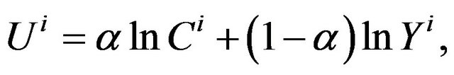
Preferences are defined over a homogeneous good, named Y, and over differentiated goods, named C. In this paper, the preferences of household  in the home country are represented by the following utility function2:
 (1)
(1)
where a is the expenditure share on differentiated goods. Here, we take the price of the homogeneous good as the numéraire. Hence, the price is normalized to one. In addition, in Equation (1), the consumption index Ci is defined as follows:
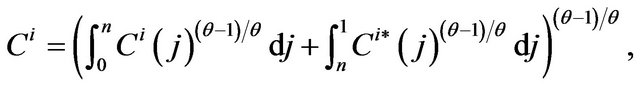 (2)
(2)
where  measures the elasticity of substitution between any two differentiated goods and
  is the consumption of good j for household i. Here, we assume iceberg transport costs in shipping the differentiated goods between countries. Specifically,
  units of a differentiated good have to be shipped from the foreign country to the home country for one unit to arrive at its destination. Similarly,
  units of a differentiated good have to be shipped from the home to the foreign country for one unit to arrive at its destination. Therefore, the asymmetry of transportation costs is characterized by
 . Then, the consumption price indices are defined as:
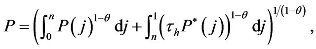 (3)
(3)
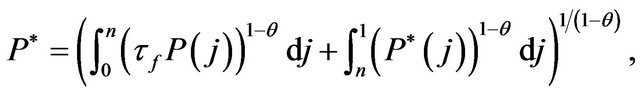 (4)
(4)
where  is the price of differentiated goods produced in j. The value of expenditure for household i, Ei, is defined as follows:
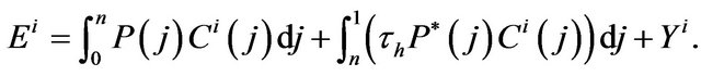 (5)
(5)
Then, the household budget constraint can be written as:
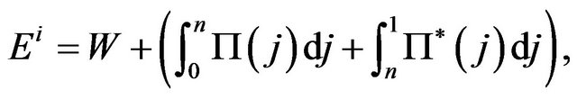 (6)
(6)
where W denotes the nominal wage rate,  is the nominal profit flow of firm j located at home (abroad).
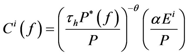
Households in the home (foreign) country maximize (1) subject to a given level of expenditure (5) by allocating differentiated goods  and Yi optimally. This problem yields:
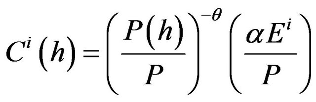 , (7a)
 , (7b)
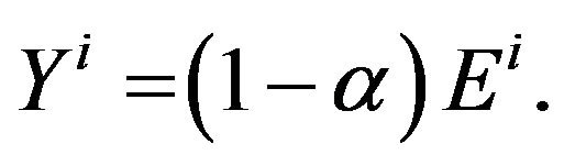 (7c)
(7c)
Here, we define  and
and  for convenience. The households are supposed to be symmetric, so we can delete the superscript i from Ei. Aggregating the demands in (7) across all households worldwide yields the following market clearing condition for any differentiated product h,
  3:
3:
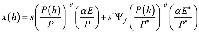 . (8)
. (8)
Similarly, for any product f of the foreign located firms, we obtain:
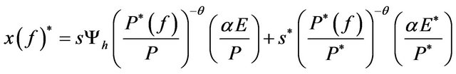 .
.
(9)
In the monopolistic goods sector, each firm has some monopoly power over pricing and one unit of labor is required to produce one unit of a variety. Because homelocated firm h hires labor domestically, given 
 and n, and subject to (8), home-located firm h faces the following profit-maximization problem:
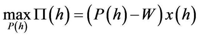 . By substituting
from Equation (8) into the firm’s nominal profit  and then differentiating the resulting equation with respect to
 , we obtain the following price markup:
 . (10)
Turning to the homogeneous good sector, one unit of labor is required to produce one unit of the homogeneous good. In addition, we assume that some production of the homogeneous good is active in both countries. Hence, the factor-price equalization across countries  is ensured because of free trade of the homogeneous good. Therefore, from (10), we obtain:
 . (11)
Substituting (8) and (10) and those of foreign counterparts into the profit flows of the homeand foreign-located firms,  and
and , respectively, we obtain:
 . (12)
The model assumes that firms do not face any relocation costs so that it does not take any time to relocate to another country. For a firm to be indifferent between home and foreign locations after location arbitrage, returns from the two locations must be equalized as follows:
 . (13)
Here, substituting (11) into (3) and (4), respectivelywe have 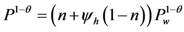 and
and
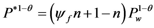 . In addition, substituting these equations and (12) into (8) and (9), respectively, we obtain:
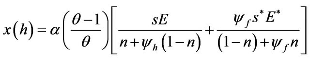 , (14)
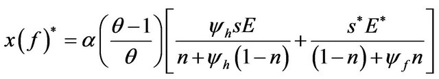 . (15)
Furthermore, from (12) and (13), we obtain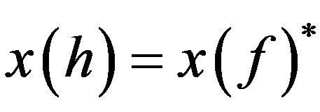 . If we substitute (14) and (15) into
 , we obtain:
 . (16)
Substituting (16) into (14) and considering , we obtain:
 , (17)
where
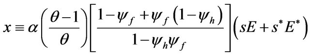 .
.
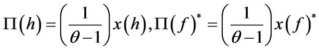
From (12), (13) and (17), we obtain:
 . (18)
By Equations (6) and (18) and because of , we have:
 . (19)
Similarly, for the foreign country, we obtain:
 . (20)
3. Market Equilibrium
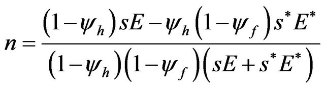
From (17), (19) and (20), we obtain:
 , (21)
where
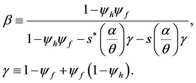
Substituting (21) into (16) gives:
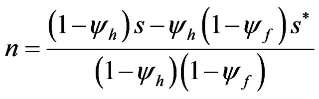 .4 (22)
From (22) and considering , we find the parametric condition required for n to be between 0 and 1 (an interior equilibrium) as follows:
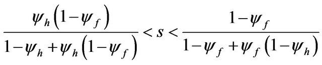 . (23)
In what follows, we assume that (23) is valid, so that both countries produce the differentiated products.
To explore the pervasiveness of HMEs in the constant returns model, following Helpman and Krugman [1], we focus on the range of parameter spaces of n and s. If n exceeds s, the HME exists, i.e., the larger country has a disproportionally larger share of firms. Conversely, if n falls below s, the result is the opposite, i.e., the larger country has a disproportionally smaller share of firms. From (22), we obtain:
 , when
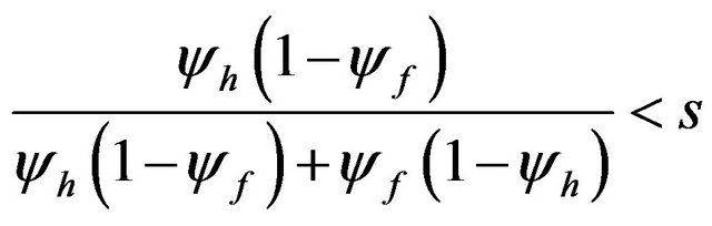 , (24)
 , when
 , (25)
 , when
 . (26)
From (24), when the home country’s transportation cost is large enough (large th or small yh) for a given level of tf, the HME appears in the home country. Meanwhile, Equation (26) shows that the opposite of the HME is observed in the home country as long as the foreign country’s transportation cost is large enough (large tf or small yf) for a given level of th. The above results imply that whether our model with asymmetric transportation costs can exhibit the HME or the opposite effect of the HME depends on the relative size of the transportation cost between the home and foreign countries.
Next, we consider the relationship between the asymmetric transportation costs and the equilibrium share of firms. Here, for simplicity, we assume . Therefore, if n exceeds
 , the home (foreign) country has a disproportionally larger (smaller) share of firms. Conversely, if n falls below
 , the result is the opposite, i.e., the home (foreign) country has a disproportionally smaller (larger) share of firms. From (22), we obtain:
 , when
 , (27)
 , when
 , (28)
 , when
 . (29)
From the above results, if the home country’s transportation cost is larger (smaller) than the foreign country’s transportation cost, then the home country ends up with a disproportionately high (low) share of firms. This is because an increase in th (or a decrease in yh) leads to  and thereby induces some firms to relocate into the home country. Thus, the country that has the larger transportation cost ends up with a disproportionately high share of firms. In contrast, the country that has the smaller transportation cost ends up with a disproportionately low share of firms.
4. Concluding Remarks
A considerable number of recent theoretical studies have examined the robustness of the HME based on the assumptions of symmetric transportation costs and increasing returns to scale technology. This paper analyzed whether or not the model exhibits the HME after removal of these assumptions using a monopolistic competition model with asymmetric transportation costs. The results indicate that when the home country’s transportation cost is large enough for a given level of the foreign country’s transportation cost, the HME appears in the home country. In addition, we also find that the opposite of the HME is observed in the home country as long as the foreign country’s transportation cost is large enough.
5. Acknowledgements
I would like to thank an anonymous referee for helpful comments and suggestions. The author is grateful to have received financial support from Tezukayama University.
REFERENCES
- E. Helpman and P. Krugman, “Market Structure and Foreign Trade,” MIT Press, Cambridge, 1985.
- D. R. Davis, “The Home Market, Trade, and Industrial Structure,” American Economic Review, Vol. 88, No. 5, 1998, pp. 1264-1276.
- K. Head, T. Mayer and J. Ries, “On the Pervasiveness of Home Market Effects,” Economica, Vol. 69, No. 275, 2002, pp. 371-390. doi:10.1111/1468-0335.00289
- Z. Yu, “Trade, Market Size, and Industrial Structure: Revisiting the Home-market Effect,” Canadian Journal of Economics, Vol. 38, No. 1, 2005, pp. 255-272. doi:10.1111/j.0008-4085.2005.00279.x
- M. Larch, “The Home Market Effect in Models with Multinational Enterprises,” Review of International Economics, Vol. 15, No.1, 2007, pp. 62-74. doi:10.1111/j.1467-9396.2007.00673.x
- M. Crozet and F. Trionfetti, “Trade Costs and the Home Market Effect,” Journal of International Economics, Vol. 76, No. 2, 2008, pp. 309-321. doi:10.1016/j.jinteco.2008.07.006
- K. Behrens, A. Lamorgese, G. I. P. Ottaviano and T. Tabuchi, “Beyond the Home Market Effect: Market Size and Specialization in a Multi-Country World,” Journal of International Economics, Vol. 79, No. 2, 2009, pp. 259- 265. doi:10.1016/j.jinteco.2009.08.005
- T. Takahashi, “Asymmetric Transport Costs and Economic Geography,” CSIS Discussion Paper, No. 87, 2007.
- V. Leite, S. Castro and J. Correia-da-Silva, “The Core Periphery Model with Asymmetric Inter-Regional and Intra-Regional Transportation Costs,” Portuguese Economic Journal, Vol. 8, No. 1, 2009, pp. 37-44. doi:10.1007/s10258-009-0036-x
- W. Johdo, “The Home Market Effect under Constant Returns and Monopolistic Competition,” Theoretical Economics Letters, Vol. 2, No. 5, 2012, pp. 441-445. doi:10.4236/tel.2012.25082
NOTES
1For related works, see Crozet and Trionfetti [6] and Behrens, Lamorgese, Ottaviano and Tabuchi [7].
2In what follows, we focus mainly on the description of the home country because the foreign country is described analogously.
3We have used the index h to denote the symmetric values within the home country, and we have used the index f for the foreign country.
4From (22), the symmetric equilibrium n = 1/2 is always a solution when (h (= (f and s (= s* = 1/2.