ABSTRACT

This paper provides a proof that the well-known quadratic Mincer (1974) Equation, wherein the log of wage or salary is a quadratic function of the years of experience, is inconsistent with the usual assumptions of utility maximization. The proof requires the use of the dynamic version of the Mincer Equation and the assumption of an isoelastic marginal utility function. The result is that a polynomial of degree three or greater is required to relate the log of wage or salary to the number of years of experience.

1. Introduction

The traditional Mincer [1] curve yields the convenient result that the log of wages or salary (henceforth wage) is a quadratic function of the years of experience. Murphy and Welch [2], however, found that making the log of wages a second degree polynomial function of experience often provides only a weak explanation of the data. This has also been found, by the current authors, to be the case for professional salaries such as lawyers, doctors and CPAs. In particular the quadratic function tends to underestimate the log of wages early in the career and overestimate the log of wages in the mid to later years. Murphy and Welch find that replacing the second degree polynomial with a third degree or higher polynomial greatly improves the estimated relationship. There is little theoretical justification offered, however, for increasing the degree of the polynomial.

The famous Stone-Weierstrass [3] Theorem states that any continuous function can be approximated to any degree of accuracy by a polynomial function of finite degree. In economics, whenever an approximating function is needed, the second degree polynomial function is usually chosen. It is well known that increasing the degree of an approximating polynomial function will always improve predictions. But increasing the degree of the polynomial can also produce its own econometric problems, e.g. multicollinearity, as well as invoke the criticism that it turns the relationship being sought into an econometric “fishing trip”. If the second degree polynomial is justified, theoretically, in the original Mincer model then what is the underlying justification for adding the third degree polynomial?

In this paper it is shown that there is a simple justification for why a third degree polynomial should be used to estimate the earnings Equation, at least for occupations where individuals can optimally choose the level of continuing education (CE). The underlying characteristic of CE for professional occupations is that individuals are rewarded for CE and are free to choose their optimal utility maximizing amount along their working life-cycle, subject to a required minimum level necessary to remain certified.

2. Literature Review

The Mincer model has been modified by others over the years to account for various changes in the assumptions, (Heckman, et al., [4] and Lemieux, [5]). While the Mincer model is inherently a dynamic model since it involves a life-cycle analysis, some variations are more dynamic than others. Ben-Porath [6] provides possibly the earliest dynamic model. His model uses familiar dynamic growth Equations to model the growth of human capital stock. Wages are then related to the accumulated human capital stock. Sheshinski [7] is the first to use optimal control to determine the level of education that maximizes income over the life-cycle. Haley [8], again using optimal control, relates the amount of investment to the individual’s earning potential based on human capital stock accumulation. Ryder, et al., [9] includes the choice of leisure in the dynamic model. Haley [10], like Ben-Porath, formulates the problem as one with the embedded optimal formation of human capital stock and then estimates the parameters as a nonlinear regression problem. Leibowitz [11] shows that the “intensity of education”, based on ability, can alter the shapes of the Mincer curves. Driffill [12] modifies the earnings model by allowing the retirement age to be endogenous. Behrman and Birdsall [13] modify the Mincer model by allowing the rate of return on the investment in CE to be a function of the quality of the initial schooling. This creates subsequent effects over the working life-cycle.

In a slightly different direction there have been several attempts to determine empirically the best functional form of the relationship between wages and experience without relating it to theoretical modifications in the Mincer model. Heckman and Polachek [14] and Frazis and Loewenstein [15] both rely on actual data and a Box and Cox transformation to examine this. Heckman and Polachek conclude that the log of wages as a quadratic function of experience, i.e., that used in the traditional Mincer model, provides satisfactory results. Frazis and Loewenstein resort to a harmonic (Fourier) approximating function that can accomplish basically what approximating polynomials can do. They are, on the other hand, less familiar to most economists and do not easily reveal the sign of the second derivative of the estimated functions.

All of the above extensions or modifications of the Mincer model result in direct or implied variations in the underlying relationship between earnings and years of experience. None, however, specifically shows that the quadratic estimation of the relationship between wages and experience is inconsistent with basic theory. This paper explains why a third degree polynomial, not the quadratic, is appropriate in estimating a modified Mincer curve.

The next section is used to derive the dynamic version of the Mincer model. In section four the Mincer model is modified by allowing the individual to choose the optimal level of CE. This is followed by the conclusion.

3. The Traditional Mincer Equation

The traditional Mincer Equation models the relationship between the log of wage in period t, ln(w_t), the years of formal schooling, s, the years of experience EXPER, and the years of experience squared, EXPER²

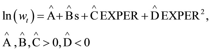(1)

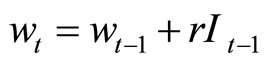
Derivation of Equation (1) has been made conveniently simple by the work of Heckman, Lochner, and Todd [16]. The initial Equation for deriving the traditional Mincer equation is:

(2)

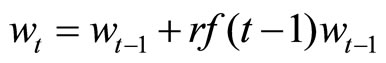
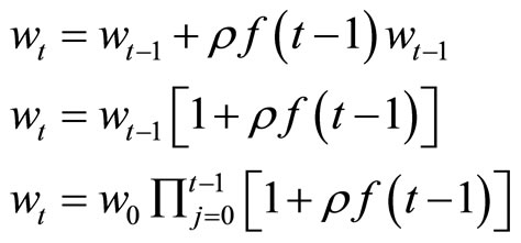
Equation (2) implies that the wage in period t equals the wage in the previous period plus some return, r, on the investment in CE in the previous period,. It is important to note that the investment in CE is not just the explicit cost of taking additional courses in formal education. The additional, perhaps primary, cost for the types of professions under consideration is the opportunity cost of time whenever one chooses to give up immediate income-earning activities in order to make future efforts more productive. Some types of investment in the future are not easily measured, at least directly, but the opportunity cost of time is proportional to the current wage and, as such, it is an important part of the Mincer Equation.

The level of investment in continuing education in the previous period is assumed to be dependent on where the individual is located within his or her working life-cycle, t < T, where T is the retirement period and t is the current period and also the current years of experience. The level of investment at any time t is defined as a fraction of the share of current wage, f, devoted to continuing education. This fraction changes systematically along the working life-cycle and thus is a function of the amount of working experience, or. In this paper it is convenient to refer to as the “CE function”. In the discrete case the fraction of wage in the previous period determines the level of investment in the previous period. This is written as the simple product:

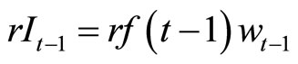(3)

Substitution of Equation (3) into Equation (2) produces:

(4)

Alternatively as the intervals in time become short relative to the entire working period T, Equation (4) can be rewritten as a continuous time Equation:

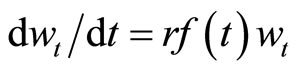(5)

Thus in this model the change in wages is totally dependent on investment in education. Certainly other things can be involved but the goal here is to focus only on the original Mincer assumptions. Equation (5) can also be written as:

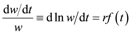(6)

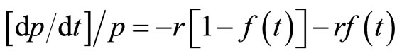
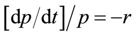
The growth rate in wages depends only on the fraction of current wages used for investment in education and the return on this investment.

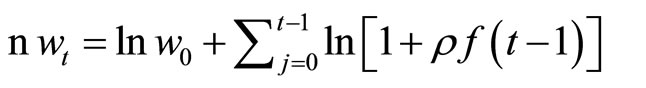
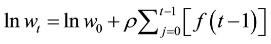
Integration of (6) yields the following Equation:

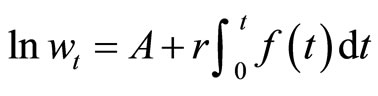(7)

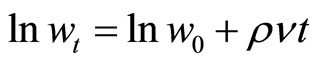
The traditional Mincer Equation imposes a specific functional form on as it changes with experience over the working life-cycle. The assumption is that is a negatively sloped linear function of time. The function is a large fraction of one’s current wage at the beginning of the career, when t is low. This implies that when individuals are just beginning their careers they choose an investment in further education that is a significant portion of their current wage, knowing that they have until retirement, T, or years, to reap the benefits. Also their wages are lower in the early years and the fixed cost of CE might be a larger portion of the current wage. As time t increases, individuals logically choose to allow the fraction to decrease since there is less time to reap the benefits. The CE function for the traditional Mincer Equation is:

(8)

where , and s = the years of full-time formal education (see Appendix A for derivation). Thus f(t) is assumed to be linear with a negative slope so that and for the traditional Mincer Equation.

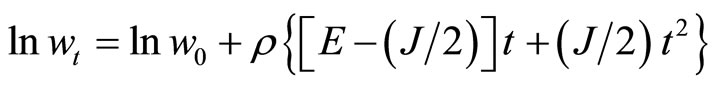
Substitution of Equation (8) into Equation (7) and integration over t yields the well-known quadratic relationship equivalent to that shown in Equation (1), or:

(9)

4. Optimal Amount of Continuing Education

The traditional Mincer Equation imposes a decreasing linear functional form on the CE function,. This is reasonable as a first approximation, but an exact form of the function, , should be derived from an optimization approach. In this case linearity is seldom the optimal solution.

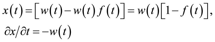
As the above literature review indicates, there are many variations in the optimal choice problem facing the professional. The most basic decision is that of holding onto one’s wealth or investing it in further CE that can provide more income in the future. The individual’s utility, U, at any time t is assumed to be a function of his or her wage at that time minus the investment in CE. The return from additional CE is enjoyed in a later period. Let, be the net wage after investment in CE. The individual’s utility function is given by:

(10)

For simplicity the utility function is not an explicit function of time.

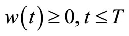
The problem of choosing the optimal amount of x(t) at each point of time, and therefore the optimal amount of CE, can be formulated as a standard optimal control problem with fixed time, T, and unspecified. The problem is written as:

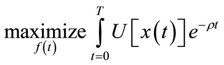(11)

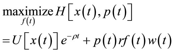
Subject to the differential Equation (5). The Hamiltonian is written as:

(12)

with,. The costate variable is the discounted marginal utility of x(t) due to an increase in gross wages.

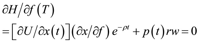
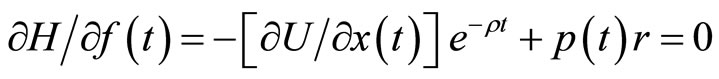
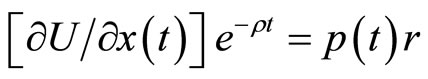
The optimal control conditions for an interior solution, along with Equation (5), are:

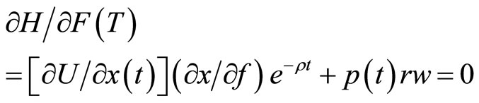(13)

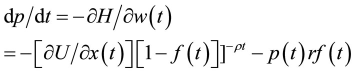(14)

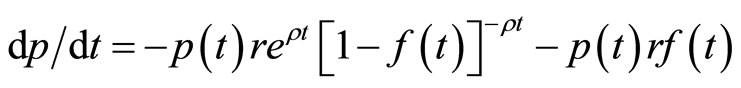
Combining Equations (13) and (14) yields a relationship that holds for all utility functions (see Appendix B):

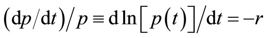(15)

Equation (15) implies that the growth rate of the discounted marginal utility of current wage is negative and equal to the negative of the return on further education. Thus decreases over the working life cycle but at a constant rate. The negative growth rate in the discounted marginal utility of is negatively proportional to the return on the investment in future wages. A higher return on the investment in education, and thus future wages, decreases the growth rate in the discounted marginal utility of.

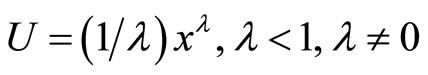
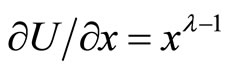
While others have formed the above optimal control problem, it is essential to seek an explicit solution to the optimal CE function,. In order to do this a specific utility function must be assumed. One familiar utility function used in dynamic models is the isoelastic (marginal) utility function:

(16)

where: (bounded utility), (Bernoulli log utility), and (unbounded utility) and is Pratt’s measure of relative risk aversion.

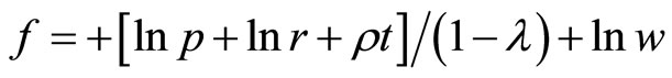
Using the optimization conditions of Equations (13)- (15) along with the utility function given by Equation (16), the optimal CE function can be derived (see Appendix B for complete derivation):

(17)

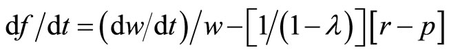
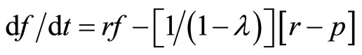
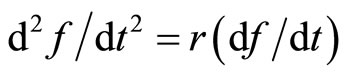
In Equation (17) as the parameter λ decreases, the CE function decreases and the individual tends to choose more current consumption over future consumption. Of interest here are the first and second derivatives of the CE function with respect to time. Taking the derivative of with respect to time in Equation (17) and making use of both Equations (5) and (15) the following derivatives are obtained

(18)

(19)

The traditional Mincer Equation embodies the assumption that the first derivative of is negative and the second derivative is zero, i.e., the function is linear with a negative slope. For and in Equation (18) it requires that r > ρ, i.e., the return to CE is greater than the personal discount rate. This is the generally accepted assumption in such models. From Equation (19) it can be seen that if df/dt < 0, then it must be true that. The implication is that if it is optimal to decrease the CE function over time, then it is optimal to decrease CE at an increasing rate, not at a constant (linear) rate as in the traditional Mincer Equation. Thus the continuing education function is assumed to be negatively sloped but concave from below during the earlier stages of the professional’s career.

Estimating the CE function with a polynomial function when it is concave from below rather than linear requires a quadratic (second degree polynomial) function, not a linear function. But this implies that estimating the log of wage as a function of experience, i.e., the integral of the CE function, requires a third degree polynomial, not a second degree polynomial as in the traditional Mincer Equation. Thus whenever researchers report that the traditional Mincer curve fails to explain wages, it is not just expedient but theoretically consistent that they increase the polynomial from second degree to a third degree. Increasing the degree of a polynomial Equation used for estimation purposes will, of course, always improve its explanatory power. But there should be a justification for adding degrees to a polynomial. Whenever individuals can make their own optimal choice of CE, the log of wage should be explained by a third degree polynomial, not the quadratic.

It should be also noted that if there is a minimum CE requirement the concave from below CE function must eventually become concave from above in the later years of the working life-cycle. In this case the log of wages would be a 4^th degree polynomial function of the years of experience.

5. Conclusion

In this study a proof is provided that demonstrates that the quadratic Mincer Equation is inconsistent with the generally accepted view that there is a diminishing marginal utility of net income (after investment in continuing education). The proof depends on the assumption that individuals will choose their own optimal level of continuing education (CE) over their working life-cycle. This results in a functional relationship that has a negative second derivative in the continuing education function with respect to time. This, in turn, implies that if a polynomial function is used to estimate the earnings Equation it should be at least a third degree polynomial function of experience, not the traditional quadratic function. Our results provide a theoretical justification to the empirical findings of Murphy and Welch (1990).

REFERENCES

Appendix A

In this appendix Equation (8) is derived:

(A1)

Taking the log of both sides:

(A2)

Using the relationship

where and for r > 1, Equation (A2) can be written as:

(A3)

If where and for the standard Mincer Equation then (A3) can be rewritten as:

(A4)

Since then:

(A5)

On the other hand if, then Equation (A2) yields:

(A6)

Appendix B

Here Equations (18) and (19) are derived. Begin with the assumption:

(B1)

with, , , and from Equation (6):

(B2)

The optimal conditions for an interior solution are:

(B3)

and:

(B4)

Given:

(B5)

using (B5), (B3) can be rewritten as:

And thus:

And finally:

(B6)

Now combining (B4) and (B6):

or:

Yielding:

(B7)

Equation (B7) holds true for all utility functions.

Therefore assume there is an isoelastic (marginal) utility function:

(B8)

(B9)

Using (B9) in (B6):

and from the definition (B5):

Taking the natural log of both sides:

or

But for, a simplification also used in the derivation of the original Mincer Equation. Thus:

(B10)

and:

(B11)

Substituting (B2) into (B11) results in:

(B12)

and:

(B13)

If it implies that.

REFERENCES

- J. Mincer, “Schooling, Experience and Earnings,” Columbia University Press, New York, 1974.
- K. Murphy and F. Welch, “Empirical Age-Earnings Profiles,” Journal of Labor Economics, Vol. 8, No. 2, 1990, pp. 202-229. doi:10.1086/298220
- M. Stone, “The Generalized Weierstrass Approximation Theorem,” Mathematics Magazine, Vol. 21, No. 4, 1948, pp. 167-184. doi:10.2307/3029750
- J. Heckman, L. Lochner and P. Todd, “Fifty Years of Mincer Earnings Regressions,” NBER WP 9732, 2003.
- T. Lemieux, “The Mincer Equation, Thirty Years after Schooling Experience, and Earnings,” Center for Labor Economics, University of California-Berkeley, Berkeley, 2003.
- Y. Ben-Porath, “The Production of Human Capital and Life Cycle of Earnings,” The Journal of Political Economy, Vol. 75, No. 4, 1967, pp. 352-365. doi:10.1086/259291
- E. Sheshinski, “On the Individual’s Lifetime Allocation Between Education and Work,” Metroeconomica, Vol. 20, No. 1, 1968, pp. 42-49. doi:10.1111/j.1467-999X.1968.tb00123.x
- W. J. Haley, “Human Capital: The Choice between Investment and Income,” American Economic Review, Vol. 63, No. 5, 1973, pp. 929-944.
- H. Ryder, F. Stafford and P. Stephan, “Labor, Leisure and Training over the Life-Cycle,” International Economic Review, Vol. 17, No. 3, 1976, pp. 651-674. doi:10.2307/2525794
- W. Haley, “Estimation of the Earnings Profile from Optimal Human Capital Accumulation,” Econometrica, Vol. 44, No. 6, 1976, pp. 1223-1238. doi:10.2307/1914256
- A. Leibowitz, “Years of Intensity of Schooling Investment,” American Economic Review, Vol. 66, No. 3, 1976, pp. 321-334.
- J. Driffill, “Life-Cycles with Terminal Retirement,” International Economic Review, Vol. 21, No. 1, 1980, pp. 45-62. doi:10.2307/2526239
- J. Behrman and N. Birdsall, “The Quality of Schooling: Quantity Alone Is Misleading,” American Economic Review, Vol. 73, No. 5, 1983, pp. 928-946.
- J. Heckman and S. Polachek, “Empirical Evidence of the Functional Form of the Earnings-Schooling Relationship,” Journal of the American Statistical Association, Vol. 69, No. 346, 1974, pp. 350-354. doi:10.2307/2285656
- H. Frazis and M. Loewenstein, “Reexamining the Returns to Training: Functional Form, Magnitude, and Interpretation,” The Journal of Human Resources, Vol. 40, No. 2, 2005, pp. 453-476.
- J. Heckman, L. Lochner and P. Todd, “Earnings Functions, Rates of Return and Treatment Effects: The Mincer Equation and Beyond,” In: E. Hanishek and F. Welch, Eds., Handbook of the Economics of Education, Elsevier, Amsterdam, 2006, pp. 307-458. doi:10.1016/S1574-0692(06)01007-5