ABSTRACT

The design of this study is to investigate the evolution of a stochastic price process consequent to discrete processes of bids and offers in a market microstructure setting. Under a set of flexible assumptions about agent preferences, we generate a price process to compare with observation. Specifically, we allow for both rational and irrational economic behavior, abstracting the inquiry from classical studies relying on utility theory. The goal is to provide a set of economic primitives which point inexorably to the price processes we see, rather than to assume such process from the start.

1. Introduction

We propose to model a price process based on microstructural activity of a market. We assume a set of agents such that each agent at any moment has both bid and ask prices present in the market. A trade occurs if and only if the bid of one agent is equal to the ask of another, this common value becoming the price of a trade. We calculate the dynamics of the resulting price process, including the moments of trades, in a discrete time setting for behavioral choices of the agents. These choices are formalized in relevant probability distributions specific to the agents’ behaviors. In this way, we allow for a multitude of behavioral patterns, including, but not restricted to traditional motivations inspired by utility functions. Our model is flexible enough to allow for “marks” to a trade, ancillary data such as its time stamp, so that we may study independently such features as trade clustering and time deformation.

Recent history is rich with microstructure studies of financial markets and with associations of specific families of probability distributions to financial stochastic processes. For good reviews of the microstructure literature see these works respectively [1,2]. For associations of probability distributions such as the widely applied Gaussian, normal inverse Gaussian, and more inclusively the generalized hyperbolic, see these studies [3,4]. In many instances such inquiries assume at the outset various forms of stochastic processes, as defined by stochastic differential equations, and then set forth to estimate parameters. Popular choices are Itô diffusions and Ornstein-Uhlenbeck processes, with and without the superposition of pure jump Lévy processes.

Most studies of microstructure take an econometric approach, that is, they define some structure, assume distributions as appropriate, then estimate parameters using data. In his survey with important bibliography, Bollerslev reviews the state of financial econometrics [5]. In a subsection discussing time-varying volatility, he notes that, “several challenging questions related to the proper modeling of ultra high-frequency data, longer-run dependencies, and large dimensional systems remain.” Further in the text, he qualifies this remark by stating: “Not withstanding much recent progress, the formulation of a workable dynamic time series model which readily accommodates all of the high-frequency data features, yet survives under temporal aggregation, remains elusive.”

Engle provides just such an econometric study [6] employing the Autoregressive Conditional Duration (ACD) model developed by him with Russell [7] in the study of IBM stock transactional arrival times. In the former paper, Engle, in referring to cases of the conditional duration function, relates, “In each case, the density is assumed to be exponential.” Such assumptions are typical, and necessary, for an econometric study focusing on time series of prices as the fundamental data structure.

Hasbrouck, in focusing on the refinement of bid and ask quotes, proposes and estimates an Autoregressive Conditional Heteroskedasticity (ARCH) model using Alcoa stock transactions, evenly spaced at 15 minute intervals [8]. Routinely, he asks the reader to consider, “a stock with an annual log return standard deviation of 0.30” The reference “return” is of course to the price sequence, a necessary expedient in the classical econometric framework which considers a price process as fundamental, rather than consequential to a set of underlying bid and ask processes.

Other studies, such as one by Bondarenko, delve into the bid and ask series, but rather as a difference, the spread [9]. The focus of this work and its principal results are in the realm of market liquidity, rather than in the estimation of the price process. Once again, the classical framework requires an assumption on the distribution of the price process, as evidenced in this remark made within the context of evaluating a price change between periods. “The asset’s final value is denoted, a normal random variable with mean and variance.”

Yet further studies attempt to develop directly a price process from first principles. An interesting and provocative example is a paper by Schaden, which formulates conclusions from financial analogues to fundamentals of quantum physics [10]. As he observes in the introduction, “At this stage it is impossible to decide whether a quantum description of finance is fundamentally more appropriate than a stochastic one, but quantum theory may well provide a simpler and more effective means of capturing some of the observed correlations.” Indeed, though the basic process investigated is yet a price process, not those of bids and asks. The analysis is grounded on five at first qualitative assumptions about the market, and concludes with the assertion that the evolution of prices follows “the lognormal price distribution.” In this setting it is difficult to discern how a different—and more realistic—distribution could emerge without changing substantially the assumptions, or the physics. For further background reading see [11-13].

In our paper we choose to move to a more basic level of explanation, to specify the market mechanisms among interacting agents, and then to let the model determine the price process and its features. In this way we derive such features as the distributions of prices, rather than assuming them ab initio.

We now proceed forthwith to present our case.

2. Specification of the Model

We consider for simplicity the model of the market for one stock in discrete time ¹. It is reasonable to assume that in each time there are only finite number of agents taking part in the trading on the market. Let be the number of all agents which have ever taken part in trading. At each moment the agent number i, proposes a bid price and an ask price for a goods on the market. We assume that. It is convenient to set and if at the moment the -th agent does not take part in the trading. Supposing the rational behavior of agents on the market we have, where and. We say that there is a trade between -th and -th agents at moment if or . It means that there is a trade between agents with minimal ask price and maximal bid price provided that they are equal. In order to escape some pathological examples we always assume that at every time t there exist two different agents, say number i and j, i ≠ j, such that and. In the case when more than one of the agents have the same minimal ask price and maximal bid price, say and, we suppose that a trade occurs between agents with numbers and, where.

The bids and asks can be changed only by the agents. It may happen that after such changing of prices. In order to avoid such possibilities we suppose that bid prices can be changed by agents only at even moments and ask prices only at odd moments. Nevertheless the trades can occur at any moment: even or odd.

How should the bid and ask prices change? The rules of changing bid and ask prices by the agents are different for each agent and they are based on different reasons; for instance: aims of agents, interpretations of information, personal reasons, and so on. If these prices are changed at time when a trade occurs, say between the i-th and j-th agents with prices, then the respective ask price will be not less then the price before the trade. Therefore we can say that

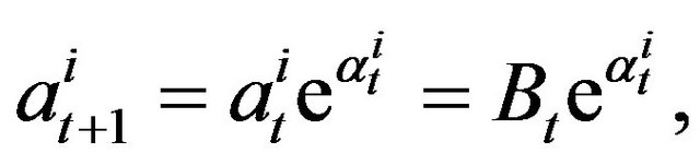
where is a nonnegative random variable (it is possible to add one more value if the agent decides to leave the market). For the bid prices we can write similarly

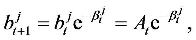
with nonnegative random variable (with the same note about). The random variables and are - and -adapted, respectively, where and are -fields containing information which the agents know before the time, inclusively. Note that and are defined only at the moment of trades.

As in the previous case we can write the same equalities for a moment when the respective agent was not involved in a trade. Hence for any we have

(2.1)

where and, are nonnegative random variables. The moment and the price of the last trade before time inclusively are given by

(2.2)

Set and.

The purpose of present paper is to calculate the distributions of and from Equation (2.2) by using the known distributions of and from Equations (2.1).

Taking min and max in Equations (2.1) yields

(2.3)

where 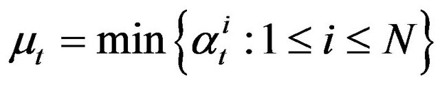and

are nonnegative random variables. Notice that and are -measurable, where is information known to at least one agent before time, inclusively.

Let us consider two nonnegative random processes and. From Equalities (2.3) we deduce that

(2.4)

(2.5)

Since the trade occurs at the moment if and only if or, equivalently, if, then the last moment of a trade before the time

(2.6)

is the last moment before when the process reached the level 1. The price of the last trade before the time is given by

(2.7)

Now the problem is reduced to finding the law of random time given by (2.6) and the law of the process given by Equation (2.4) at the time.

3. Simplest Behavior of Agents

Since the bid prices can be changed by the agent in even moments only, then. Therefore from Equation (2.3) we deduce that

(3.1)

Similarly and

(3.2)

Then Equations (3.1), (3.2) and (2.5) imply that and. Moreover, we have and. Define a new sequence by for and if,. Then, and . Hence the trade occurs at time if and only if.

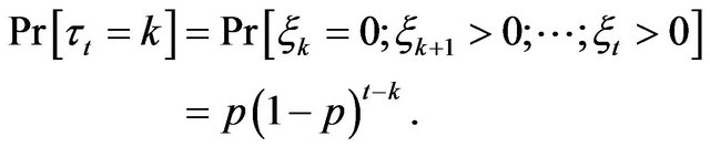
In order to obtain some result we need to have more assumptions on the behavior of the processes and. The simplest assumption is that, is a sequence of independent identically distributed (i.i.d.) random variables. Denote by p the probability that takes value zero:. The variable is a last zero of the sequence before the moment. We put if there are no zeros (no trades) before time, inclusively. Hence takes values. The probabilities of these values are given by

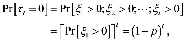
and for

Let, denote the number of trades before time t inclusively. Hence is number of zeros in the sequence,. Then has a binomial distribution with parameters and, i.e.,

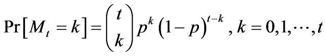
here is a binomial coefficient.

Moreover has a binomial distribution with the same parameters and. As a consequence of independence of the variables we get that for any the random variables are independent.

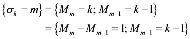
Define the sequence, of random times inductively by the following expression.

with and. We adopt the convention that the infinum of empty set is equal to infinity. Then, is a moment of -th trade (or zero of the sequence) and

for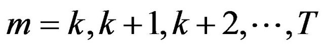. Easy calculation shows that

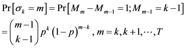
and

.

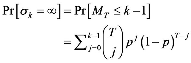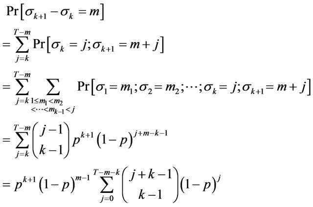
Furthermore for all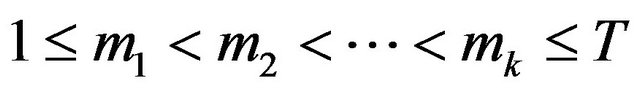, we have

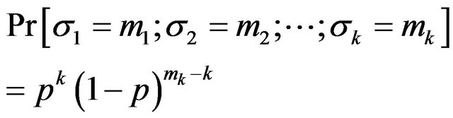
and

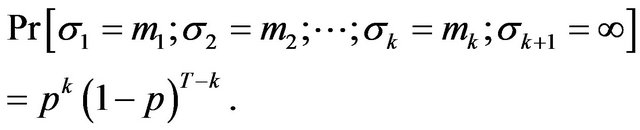
For any and we have

and

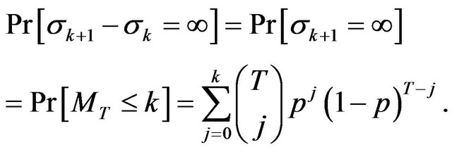
In the same way one can obtain

Notice that

.

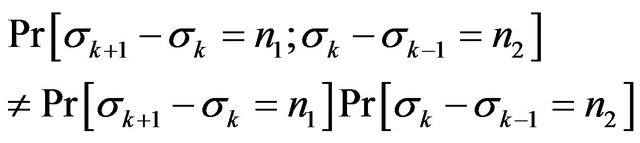Hence and are not independent.

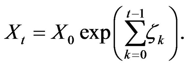
Let us consider process given by Equation (2.4). The solution of this equation can be written as

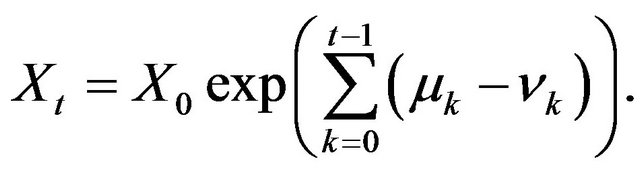(3.3)

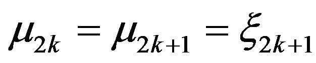Since and then

where denotes the integer part of number.

Therefore taking into account that one has

(3.4)

From the Equation (3.4) and definition of and we obtain the prices and of the last trade and the -th trade:

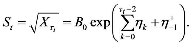
(3.5)

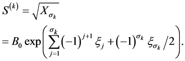(3.6)

Now we calculate the characteristic function of the logarithm. It follows from representation (3.5) that

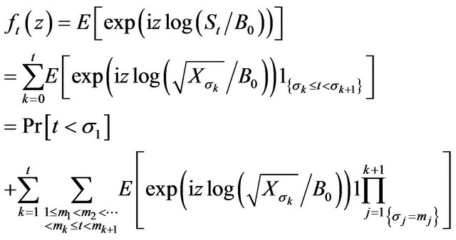
Notice that event occur if and only if and if does not coincide with some of the. This fact, formula (3.5), independence and the distribution of imply

where 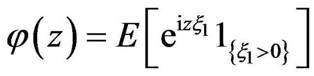is the characteristic function of conditioned on. From the relationships and we have

(3.7)

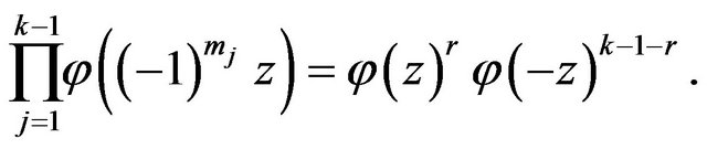
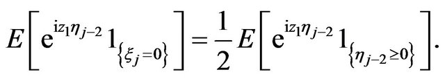
Notice that if only numbers of are even then

Therefore

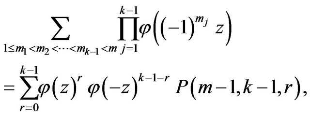
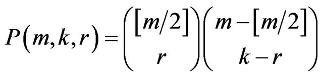
where is a number of possibilities to choose even and odd numbers from the set. Here. There are only even and odd numbers among. Hence

if or and

if and

. Putting this expression into the Formula (3.7) yields

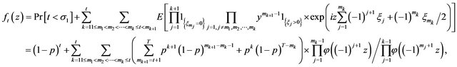
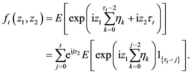
Using equation (3.6) one can compute joint characteristic function of the moment of the first trade and the logarithm provided there was at least one trade, in the following way

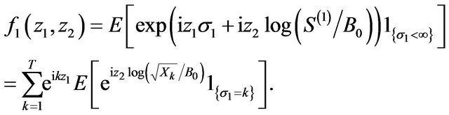
Since and the random variables 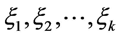are independent then

(3.8)

where is defined above. The relationships and imply

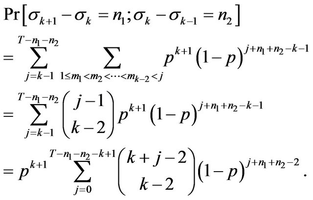
Similarly we can find joint characteristic function of the difference between moments of -th and -st trades, and the logarithm of the ratio between these trades provided there were at least trades, ,.

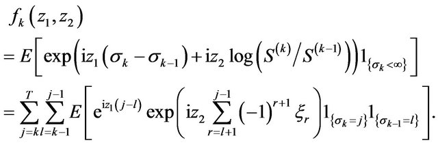
Since 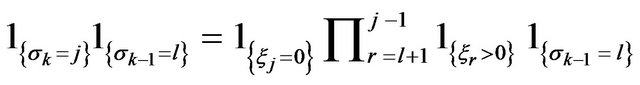and all multipliers here are independent then

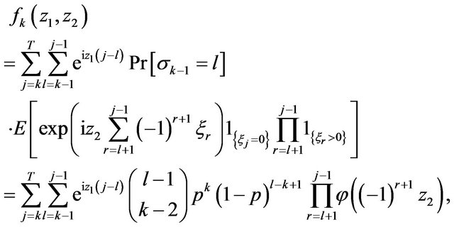
where as above. After the changing the order of summation and summation indexes we have

The same arguments as after Equality (3.8) lead to the following expression

Now we consider one more simplest case.

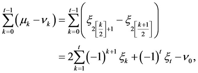
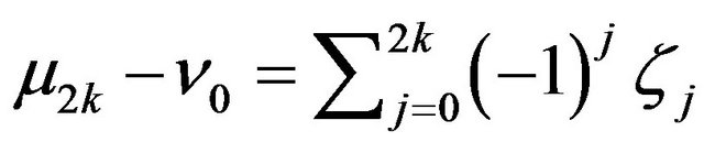
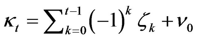
Recall the expressions for, and.

where, for and if,.

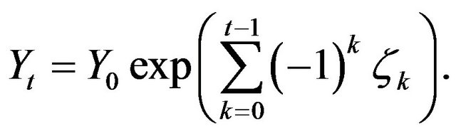
Assume that is a sequence of independent random variables. Then the power of exponent in the expression for is a random walk and is a discrete analogue of geometrical Brownian motion, which is classical choice for modeling of the price process. But in our model the price process describes by, geometrical random walk computed at random time and the distributions of and can be completely different. We show that indeed this is the case and the distribution of is trivial.

Denote: then we have

Since and then

and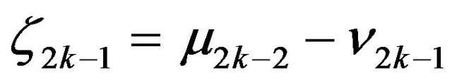. Therefore

and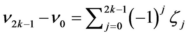

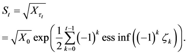
which implies the following equality:

(3.9)

From the meaning of process we have for all hence for any a.s. satisfy the following system of inequalities

Denote the left side of the last inequality by

. Then 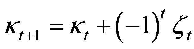and

for all. It is evident that the random variables and are independent and if and only if.

The following technical lemma will be needed.

Lemma 3.1. Let and be two independent random variables. Then

Proof. Recall the formula for distribution function of the sum of two independent random variables and

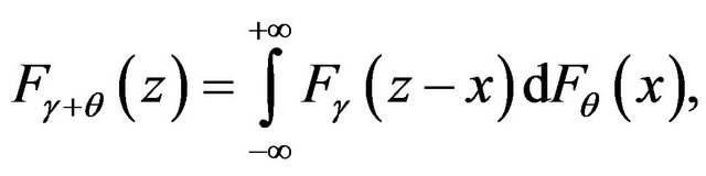
where is the distribution function of the random variable. Since for all then

for all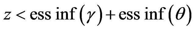. This implies that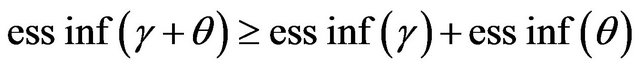. Since the opposite inequality is obvious then we have the statement of the lemma.

It follows from the non-negativity of and lemma above that for all

The trade occurs at time if and only if, i.e. when the last inequality becomes in fact equality. In this case we have that for any

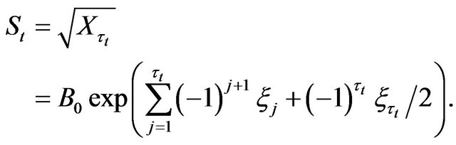
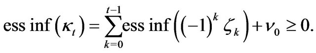
. Therefore

And the price of the last trade is deterministic and is equal to the following expression

In particular, if for all

then 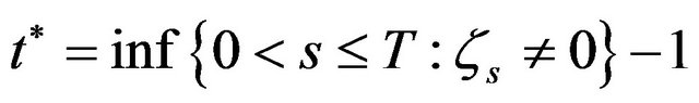is a last possible moment of trade. There is a trade at each time with the same price and there are no trades at all after the moment.

4. The Connection to Continuous Time Analogue of the Model

In this section we give an example of the agents’ behavior such that the geometrical Brownian motion can be regarded as the limit of the price process with discrete time. For this purpose let be a sequence of random variables describing the state of the real world (noise sequence). Assume that at each time the agents make their decisions about how to change bid or ask prices according to the history of the noise sequence before the present time. For instance and. The simplest case, with agents taking into account only the present value of noise was considered above.

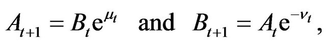
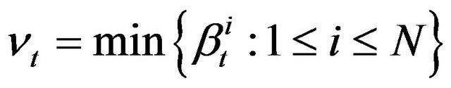
Now we consider the case when the agents are taking into account only the present and previous information, and for even and odd moments. Assume that is a sequence of independent identically distributed random variables and set and , where and.

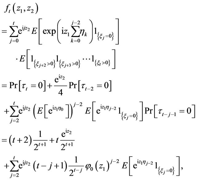
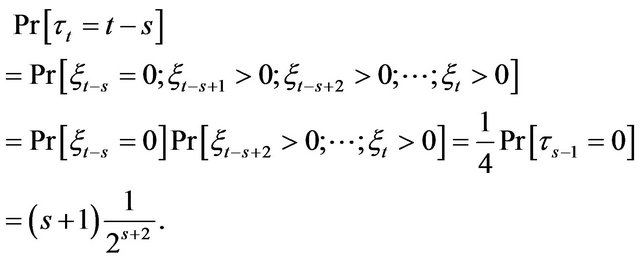
For such and we can compute the distribution of. For simplicity assume that . If there are no trades then

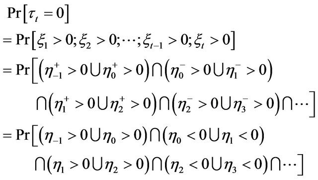
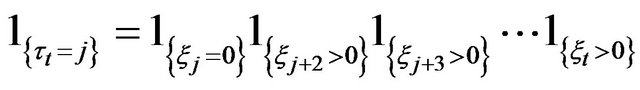
The last event happens if and only if the following condition is satisfied: for all at least one of the numbers and is positive and for all at least one of the numbers and is negative. If and have the same sign then the sign of other, satisfying the condition above is uniquely determined. The condition above is also satisfied if and have the different signs for all. Hence the number of possible choices of signs of satisfying condition above is equal to, where is a number of choices of such that and have the same sign and is number of possibilities that and have the different signs for all. Since for any choice of signs of the probability is equal to then we get

Notice that if then and a.s. Indeed, for even we have 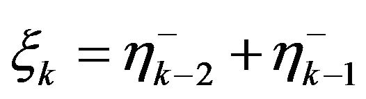and since then a.s. For odd the proof is the same. The fact that if can be shown in the same way. Hence for we get

Now consider. From Equalities (3.3) and (3.4) we have

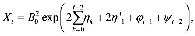(4.1)

where if and if, and if and if. Notice that the representation (4.1) is also true in the case when the random variables are not necessary independent and identically distributed. Since, then and from the last equation we deduce that

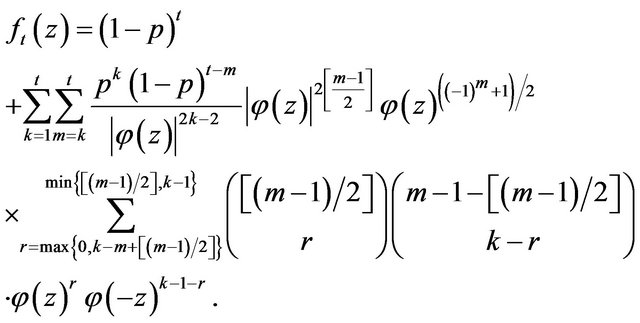
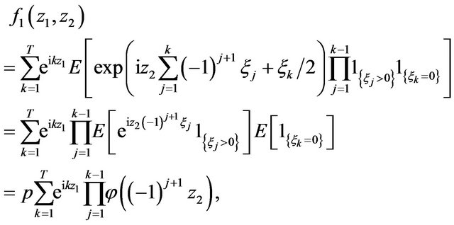
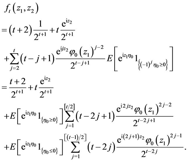
Let us compute joint characteristic function

of the sum 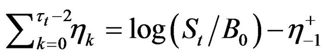and.

It has been shown above that

. Since depends on and only then

(4.2)

where is the characteristic function of.

The expression 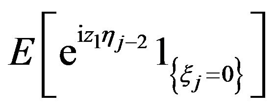can be simplified as follows. If then and

For we have 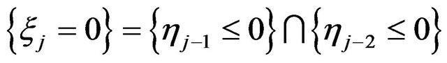. Therefore

Then the Equality (4.2) has the following form

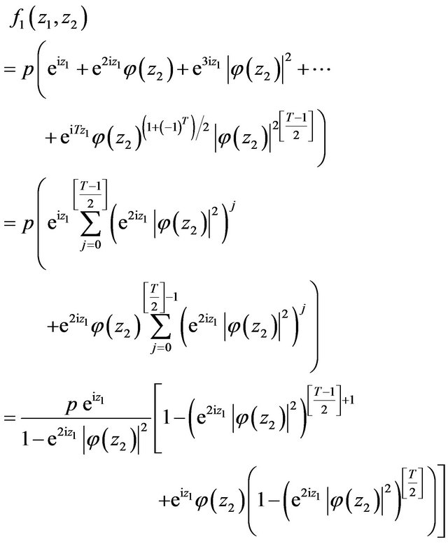
Suppose at first that. Then from the last equality we get

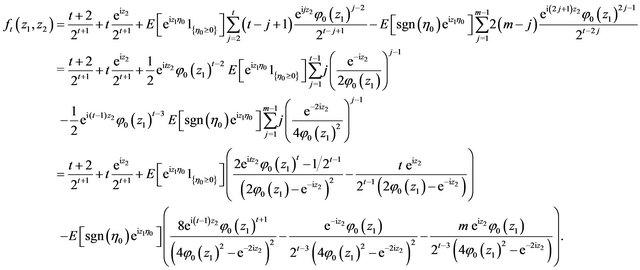
(4.3)

Similarly we have for

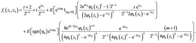(4.4)

The last Equalities (4.3) and (4.4) allow one to obtain the characteristic function of a continuous time model analogous the process as the limit of the discrete time model.

For instance, consider the partition

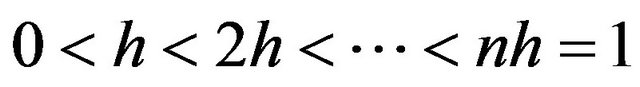of the interval. Let take values. Assume that and

, where. If the noise sequence is Gaussian, , then

Hence from (4.3) and (4.4) we have

Therefore for Gaussian noise the continuous version of price process is a geometrical Brownian motion and.

5. Conclusions

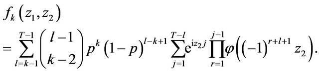
With this work we have set forth the structure for computing a price process from first principles of agent behavior in providing bid and ask quotes to a market. As well, we have provided some content by analyzing a basic case, that of a binomial assumption on the i.i.d. sequence recording the moments of trades. This assumption led to the specification of a geometric random walk computed in random time, and to the joint characteristic function of the difference

between moments of -th and -st trades, and the logarithm

of the ratio between these trades. The study culminated with an explicit expression for, and implications for a parallel model in continuous time.

Next on the agenda is to explore alternative hypotheses on agent behaviors, and to perform simulations and other numerical work as necessary to establish a theory of consequential price processes.

REFERENCES

[15]    NOTES

[16]     

[17]    ^*The work of Aleh L. Yablonski was supported by INTAS grant 03-55- 1861.

[18]    ¹For a treatment of the case wherein the duration, defined as the length of time between trades, is stochastic, see [14].

[19]

REFERENCES

- A. Madhavan, “Market Microstructure: A Survey,” Journal of Financial Markets, Vol. 3, No. 3, 2000, pp. 205- 258. doi:10.1016/S1386-4181(00)00007-0
- H. R. Stoll, Elsevier/North-Holland, Amsterdam, 2003.
- O. E. Barndorff-Nielsen, “Processes of Normal Inverse Gaussian Type,” Finance and Stochastics, Vol. 2, No. 1, 1998, pp. 41-68. doi:10.1007/s007800050032
- E. Eberlein and U. Keller, “Hyperbolic Distributions in Finance,” Bernoulli, Vol. 1, No. 3, 1995, pp. 281-299. doi:10.2307/3318481
- T. Bollerslev, “Financial Econometrics: Past Developments and Future Challenges,” Journal of Econometrics, Vol. 100, No. 1, 2001, pp. 41-51. doi:10.1016/S0304-4076(00)00052-X
- R. F. Engle, “The Econometrics of Ultra-High-Frequency Data,” Econometrica, Vol. 68, No. 1, 2000, pp. 1-22. doi:10.1111/1468-0262.00091
- R. F. Engle and J. R. Russell, “Autoregressive Conditional Duration: A New Model for Irregularly Spaced Transaction Data,” Econometrica, Vol. 66, No. 5, 1998, pp. 1127-1162. doi:10.2307/2999632
- J. Hasbrouck, “The Dynamics of Discrete Bid and Ask Quotes,” The Journal of Finance, Vol. 54, No. 6, 1999, pp. 2109-2142. doi:10.1111/0022-1082.00183
- O. Bondarenko, “Competing Market Makers, Liquidity Provision, and Bid-Ask Spreads,” Journal of Financial Markets, Vol. 4, 2001, pp. 269-308. doi:10.1016/S1386-4181(01)00014-3
- M. Schaden, “Quantum Finance,” Physica A, Vol. 316, No. 1-4, 2002, pp. 511-538. doi:10.1016/S0378-4371(02)01200-1
- S. Hermannn and P. Imkeller, “The Exit Problem for Diffusions with Time Periodic Drift and Stochastic Resonance,” Prepublication No. 01, Institut de Mathématiques Élie Cartan, Université Nancy 1, Lorraine, 2003.
- P. C. Kettler, O. M. Pamen and F. Proske, “On Local Times: Application to Pricing Using Bid-Ask,” Preprint #13, University of Oslo, Oslo, 2009. www.paulcarlislekettler.net/docs/Oliv.pdf
- G. Di Nunno, B. Øksendal and F. Proske, “Malliavin Calculus for Lévy Processes with Applications to Finance,” Universitext, 2nd Edition, Springer, Berlin, 2009.