Journal of Mathematical Finance
Vol.2 No.1(2012), Article ID:17581,12 pages DOI:10.4236/jmf.2012.21001
The Analysis of Real Data Using a Stochastic Dynamical System Able to Model Spiky Prices*#
1Dipartimento di Matematica e Informatica, Università di Camerino, Camerino, Italy
2CERI—Centro di Ricerca “Previsione, Prevenzione e Controllo dei Rischi Geologici”, Università di Roma “La Sapienza”, Roma, Italy
3Dipartimento di Scienze Sociali “D. Serrani”, Università Politecnica delle Marche, Ancona, Italy
4Dipartimento di Matematica “G. Castelnuovo”, Università di Roma “La Sapienza”, Roma, Italy
Email: lorella.fatone@unicam.it, fra_mariani@libero.it, m.c.recchioni@univpm.it, f.zirilli@caspur.it
Received October 28, 2011; revised November 25, 2011; accepted December 15, 2011
Keywords: stochastic dynamical system; inverse problem; spiky prices; data time series analysis
ABSTRACT
In this paper we use filtering and maximum likelihood methods to solve a calibration problem for a stochastic dynamical system used to model spiky asset prices. The data used in the calibration problem are the observations at discrete times of the asset price. The model considered has been introduced by V. A. Kholodnyi in [1,2] and describes spiky asset prices as the product of two independent stochastic processes: the spike process and the process that represents the asset prices in absence of spikes. A Markov chain is used to regulate the transitions between presence and absence of spikes. As suggested in [3] in a different context the calibration problem for this model is translated in a maximum likelihood problem with the likelihood function defined through the solution of a filtering problem. The estimated values of the model parameters are the coordinates of a constrained maximizer of the likelihood function. Furthermore, given the calibrated model, we develop a sort of tracking procedure able to forecast forward asset prices. Numerical examples using synthetic and real data of the solution of the calibration problem and of the performance of the tracking procedure are presented. The real data studied are electric power price data taken from the UK electricity market in the years 2004-2009. After calibrating the model using the spot prices, the forward prices forecasted with the tracking procedure and the observed forward prices are compared. This comparison can be seen as a way to validate the model, the formulation and the solution of the calibration problem and the forecasting procedure. The result of the comparison is satisfactory.
In thewebsite:http://www.econ.univpm.it/recchioni/finance/w10 some auxiliary material including animations that helps the understanding of this paper is shown. A more general reference to the work of the authors and of their coauthors in mathematical finance is the website: http://www.econ.univpm.it/recchioni/finance.
1. Introduction
A spike in an asset price is an abrupt movement of the price followed by an abrupt movement of approximately the same magnitude in the opposite direction. The modeling of spikes in asset prices is a key problem in finance. In fact spiky prices are encountered in several contexts such as, for example, in electric power prices and, more in general, in commodity prices.
In this paper the model introduced by V. A. Kholodnyi in [1,2] to describe spiky prices is combined with some ideas introduced by the authors and some coauthors to study calibration problems in mathematical finance, see [3-9]. That is we introduce a stochastic dynamical system to model spikes in asset prices and we study a calibration problem for the dynamical system introduced. The method proposed to solve the calibration problem is tested doing the analysis of data time series. We consider synthetic and real data. The real data studied are electric power price data taken from the UK electricity market in the years 2004-2009.
Following V. A. Kholodnyi (see [1,2]) we model spiky asset prices as a stochastic process that can be represented as the product of two independent stochastic processes: the spike process and the process that describes the asset prices in absence of spikes. The spike process models spikes in asset prices and it is either equal to the multiplicative amplitude of the spike during the spike periods or equal to one during the regular periods, that is during the periods between spikes. The second stochastic process of the Kholodnyi model describes prices in absence of spikes. This last process has been chosen as a diffusion process. Finally we use a two-state Markov chain in continuous time to determine whether asset prices are in the spike state, that is during a spike, or in the regular state, that is between spikes.
The model for spiky asset prices studied depends on five real parameters. Two of them come from the process that describes the asset prices in absence of spikes, one of them comes from the spike process and the last two parameters come from the two-state Markov chain used to model the transitions between spike and regular states.
The calibration problem studied consists in estimating these five parameters from the knowledge at discrete times of the asset prices (observations of the spiky prices). That is the calibration problem is a parameter identification problem or, more in general, is an inverse problem for the stochastic dynamical system that models the asset prices. This calibration problem is translated in a constrained optimization problem for a likelihood function (maximum likelihood problem) with the likelihood function defined through the solution of a filtering problem. The likelihood function is defined using the probability density function associated with the diffusion process modeling asset prices in absence of spikes. This formulation of the calibration problem is inspired to the one introduced in [3] in the study of the Heston stochastic volatility model that has been later extended to the study of several other calibration problems in mathematical finance (see [4,5,8, 9]).
The filtering and the maximum likelihood problems mentioned above are solved numerically. The resulting numerical solution of the calibration problem determines the values of the (unknown) parameters that make most likely the observations actually made. Note that in the processing of numerical data to improve the robustness and the quality of the solution of the calibration problem some preliminary steps are introduced in the optimization procedure used to solve the calibration problem and the results obtained in these preliminary steps are used to penalize the likelihood function obtained from the filtering problem. That is the maximum likelihood problem originally formulated in analogy to [3] is reformulated adding penalization terms to the likelihood function and choosing an ad hoc initial guess for the optimization procedure to improve the robustness and the quality of its solution. This reformulated optimization problem is solved numerically using a method based on a variable metric steepest ascent method.
Furthermore, as a byproduct of the solution of the filtering problem, we develop a tracking procedure that, given the calibrated model, is able to forecast forward asset prices.
The method used to solve the calibration problem and the tracking procedure are used to analyze data time series. Numerical examples of the solution of the calibration problem and of the performance of the tracking procedure using synthetic and real data are presented. The synthetic data are obtained computing one trajectory of the stochastic dynamical system that models spiky asset prices. We generate daily synthetic data for a period of two years. The first year of data is generated with one choice of the model parameters, the second year of data is generated with a different choice of the model parameters. The second year of data is generated using as initial point of the trajectory the last point of the first year of data. In the solution of the calibration problem we choose as observation period a period of one year, that is we use as data the daily observations corresponding to a time period of one year, and we move one day at the time this observation period through the two years of data. The calibration problem is solved for each choice of the observation period. The two choices of the model parameters used to generate the data and the time when the model parameters change value are reconstructed satisfactorily by the calibration procedure. The real data studied are daily electric power price data taken from the UK. electricity market. These electric power price data are spiky data. We choose the data of the calibration problems considered as done above in the study of synthetic data extracting the observation periods from a time series of five years (i.e. the years 2004-2009) of daily electric power (spot) price data taken from the UK market. The results obtained show that the model is able to establish a stable relationship between the data time series and the estimated model parameter values. Note that in the real data time series for each observation day we have the electric power spot price and the associated forward prices observed that day for a variety of delivery periods. That is for each spot price there is a set of forward prices associated to it corresponding to different delivery periods. Moreover in the calibration problem only spot prices are used as data. To exploit this fact we proceed as follows. After calibrating the model using as data the spot prices observed in the first three years of the data time series, we use the calibrated model, the tracking procedure and the spot prices not used in the calibration to forecast the forward prices associated to these last spot prices. We compare the forward prices forecasted with the tracking procedure with the observed forward prices. The comparison is satisfactory and establishes the effectiveness of the model, the validity of the proposed formulation and solution of the calibration problem and the quality of the forecasted prices.
We note that the model studied is too simplistic to be of practical value in electricity markets. In fact our model is able to capture only one property of the electric power prices: the presence of spikes. It does not consider, for example, the mean-reverting property and the presence of weekly and season cycles in electricity prices. This study aims to be a first attempt to solve, with the strategy presented in Section 3, calibration problems involving stochastic dynamical systems that can be used to describe electric power prices. That is the methodology discussed in this paper can be applied in the calibration of more sophisticated stochastic dynamical models that can be used in electricity markets (see for example [10]).
The website: http://www.econ.univpm.it/recchioni/finance/w10 contains some auxiliary material including some animations that helps the understanding of this paper. A general reference to the work of the authors and of their coauthors in mathematical finance is the website: http://www.econ.univpm.it/recchioni/finance.
The paper is organized as follows. In Section 2 we describe the model for spiky asset prices. In Section 3 we formulate and we solve the filtering and the calibration problems for the model presented in Section 2 and we introduce the tracking procedure used to forecast forward prices. In Section 4 some numerical examples of the solution of the calibration problem and of the performance of the tracking procedure introduced in Section 3 using synthetic and real data are presented.
2. The Stochastic Dynamical System for Spiky Asset Prices
Let us introduce a stochastic dynamical system used to model spiky asset prices, see [1,2]. In this model the spiky prices are defined as the product of two stochastic processes: the spike process and the process that describes asset prices in absence of spikes. As said in the Introduction the transitions between spike and regular states are regulated through a two state Markov chain in continuous time.
Let  be a real variable that denotes time,
 be the (continuous time) two-state (i.e. regular state, spike state) Markov chain and let
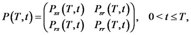 (1)
(1)
be its  transition probability matrix. Note that in (1)
  and
and  denote the transition probabilities of going from the spike state at time
  respectively to the spike or to the regular state at time
  and similarly
  and
and  denote the transition probabilities of going from the regular state at time
  respectively to the spike or to the regular state at time
Note that the Chapman-Kolmogorov equation for the Markov chain ,
,  can be written as follows:
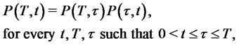 (2)
(2)
together with the condition that  is the
  identity matrix when
Let  and
and 


 be respectively the probabilities of being in the regular state and in the spike state at time
  and at time
  We have:
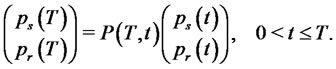 (3)
(3)
In the time-homogeneous case it is possible to write an explicit formula for the matrix ,
,  as a function of the parameters that define the generator of
 ,
,  These parameters control the duration and the frequency of the spikes, that is they control the expected lifetime of the spike periods and the expected lifetime of the periods between spikes. It is easy to see that in the case of a time-homogeneous Markov chain
 ,
,  , the transition probability matrix
 ,
,  is a function only of the difference
  and that we have [1]:
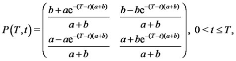 (4)
(4)
where  and
and  are non negative real parameters. Moreover we assume that
  are not both zero.
From now on in our model for spiky prices we always assume that the two-state Markov chain ,
,  is time-homogeneous and, as a consequence, we assume that its transition probability matrix
 is given by (4).
The process that describes the asset prices in absence of spikes is a diffusion process defined through the following stochastic differential equation:
 (5)
(5)
with the initial condition:
 (6)
(6)
where  denotes the random variable that describes the asset price in absence of spikes at time


 are constants,
 is the standard Wiener process,

 is its stochastic differential and the random variable
  is a given initial condition. For simplicity we assume that the random variable
  is concentrated in a point with probability one and, with abuse of notation, we denote this point with
 . Recall that
  is the drift coefficient and
  is the volatility coefficient.
Equation (5) defines the asset price dynamics of the celebrated Black-Scholes model. Note that the solution of (5), (6) is a Markov process known as geometric Brownian motion. Note that several other Markov processes different from the one defined in (5), (6) can be used to model asset price dynamics in absence of spikes. For example we can use one of the so called stochastic volatility models that have been introduced recently in mathematical finance to refine the Black-Scholes asset dynamics model.
Let us define the spike process 
 that models the amplitude of the spikes in the asset prices. Let
 be a stochastic process made of independent positive random variables with given probability density functions

 We assume that if the Markov chain
 is in the regular state then the spike process
 is equal to one. If the Markov chain
 transits from the regular state to the spike state at time
 then the spike process
 is equal to a value sampled from the random variable
  during the entire time period beginning with
  that the Markov chain
 remains in the spike state. We assume that
 is in the regular state at time
  with probability one, so that the spike process
  starts with
  with probability one. Let us observe that in the case of spikes with constant amplitude
  the probability density function

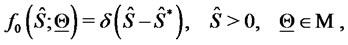
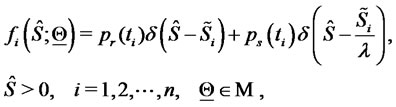
 is the Dirac delta function
  with support in
  that is we have:
 (7)
(7)
Finally we say that the spike process 
 is in the spike state or in the regular state if the Markov chain
 is in the spike state or in the regular state respectively. In our model for spiky prices we assume that the spikes have constant amplitude
  that is we assume (7).
Let us define now the process that describes the asset prices with spikes. Let us denote with  the random variable that models the price (eventually) with spikes of the asset at time
 . We assume that the spike process
 and the process
 that describes asset prices in absence of spikes, are independent. Following [1,2] we define the process
 ,
,  as the product of the spike process
 and of the process
 that is:
 (8)
(8)
Note that the process 
 for spiky asset prices is in the spike state or in the regular state depending from the fact that the spike process
 is in the spike state or in the regular state respectively, or equivalently, depending from the fact that the Markov chain
 is in the spike state or in the regular state respectively.
In [1] it has been shown that the process 
 is able to reproduce spikes in asset prices. This can be seen in Figure 1 where synthetic data sampled from
 are shown. These synthetic data are those used in the numerical examples presented in Section 4. Note that depending on the values of the parameters defining the model, the trajectories of
 can exhibit a variety of behaviours. In particular, when
 is time-homogeneous and
 the expected times
  and
and  spent by the process
 in “spike mode” and in “regular (i.e. inter-spike) mode”, respectively, are given by (see [1]):
 (9)
(9)
If  is small in comparison with the characteristic time of change of the process
 then the process
 exhibits spikes. For example, if
 is the diffusion process defined in (5) then the previous condition can be stated as follows:
 (10)
(10)
We interpret  as the expected lifetime of a spike, and
  as the expected time elapsed between two consecutive spikes. That is the parameters
  and
and  control the duration and the frequency of the spikes through (9). For example, the relations (9) suggest that in order to model short-lived spikes the parameter
  must be large, while to model rare spikes the parameter
  must
must
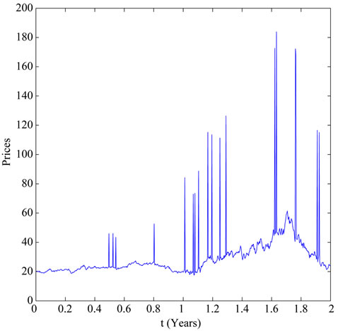
Figure 1. The synthetic data.
be small.
Using some heuristic rules to recognize spikes on the data time series considered thank to their relation with the spike duration and frequency a rough estimate of the parameters  and
and  can be obtained directly from observed spiky prices (market data). For example, the relations (9) suggest that initial estimates
  and
and  of
of  and
and  respectively, can be obtained as follows:
 (11)
(11)
where  and
and  are computed (using some heuristic rules) directly from the data available as the observed average lifetime of the spikes and the observed average time between two consecutive spikes, respectively.
Finally it is easy to see that the asymptotic probabilities of the time-homogeneous Markov chain 
 of being in the spike and in the regular states are respectively:
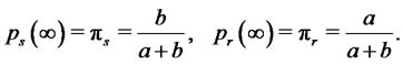 (12)
(12)
With the previous choices the model for spiky asset prices introduced in [1,2] depends on five parameters, that is:  The parameters
  and
and  are those appearing in (5) and are relative to the asset price model in absence of spikes, the remaining parameters are relative to the spike process (i.e.
 ) and to the Markov chain that regulates the transitions between spike and regular states (i.e.
 ).
).
3. The Filtering and the Calibration Problems
The parameters 


 are grouped in the following vector:
 (13)
(13)
where the superscript  denotes the transpose operator. The vector
  is the unknown of the calibration problem that must be determined from the data available. The vectors
 , describing admissible sets of parameter values, must satisfy some constraints, that is we must have
  where:
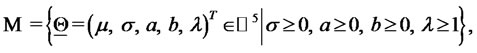 (14)
(14)
and  is the five dimensional real Euclidean space.
The constraints contained in  express some elementary properties of the model introduced in Section 2. Note that, when necessary to take care of special circumstances, more constraints can be added to
 .
.
The data of the calibration problem are the observation times:  and the spiky asset price
  observed at time
 where
where  The observed price
  is a positive real number that is understood as being sampled from the random variable
 Starting from these data we want to solve the following problems:
Calibration Problem: Find an estimate of the vector .
.
Filtering Problem (Forecasting Problem): Given the value of the vector  estimated forecast the forward asset prices.
Note that the prices 
 are called spot asset prices and that with forward asset prices we mean prices “in the future”, that is, in our setting, we mean the forward prices at time
  associated to the spot price
 ,
,  These are the prices at time
  of the asset with delivery time
 Let us point out that in correspondence of a spot price we can forecast several forward prices associated to different delivery periods. The delivery periods of interest are those actually used in real markets, in fact for these delivery periods observed forward prices are available and a comparison between observed forward prices and forecasted forward prices is possible. In Section 4 in the analysis of real data we consider (some of) the delivery periods used in the UK electricity market in the years 2004-2009 and we make this comparison.
Let us mention that the forecasted forward asset prices associated to the spiky price model introduced in Section 2 do not exhibit spikes while, of course, the corresponding (spot) asset prices exhibit spikes (see [1,2] for more details).
The calibration problem consists in estimating the value of the vector  that makes “most likely” the observations. The observations available at time
  are denoted with:
 (15)
(15)
Note that for simplicity we assume that the transitions from regular state to spike state or viceversa happen at the observation times.
Let 

 be the probability density function of the stochastic process
  at time
  conditioned to the observations
  and let


 be the probability density function of the stochastic process
  conditioned to the observations made up to time
 , when
 where for convenience we define
 .
.
The probability density functions 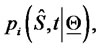

 ,
, 
 are the solutions of the following initial value problems for the Fokker-Planck equation associated to the Black-Scholes model (5):
for 
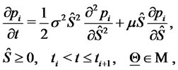 (16)
(16)
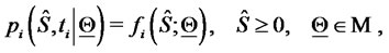 (17)
(17)
where
 (18)
(18)
 (19)
(19)
where  and
and  are, respectively, the probabilities defined through the time-homogeneous Markov chain
 of being in the regular and in the spike state at time
 (see (3)).
The probability density functions ,
,  solutions of the initial value problems for the FokkerPlanck equations (16)-(19), can be written as follows:
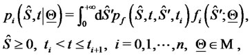 (20)
(20)
where  is the fundamental solution of the FokkerPlanck equation (16) associated to the Black-Scholes model (5), that is:
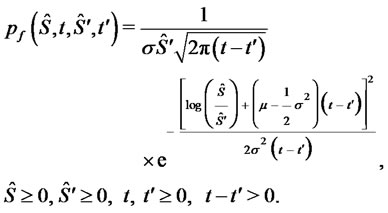 (21)
(21)
In order to measure the likelihood of the vector  we introduce the following (log-)likelihood function:
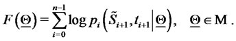 (22)
(22)
It is worthwhile to note that definition (22) contains an important simplification. In fact a more correct definition of the (log-)likelihood function should be:
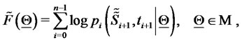 (23)
(23)
where  or
or  depending on whether at time
  the asset price is in the regular state or in the spike state respectively,
 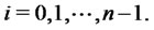 However, since when dealing with real financial data the decision about the character of the state (regular or spike state) of the observed prices is dubious, we prefer to adopt the definition (22) for the (log-)likelihood function. In fact the choice made in (22), at the price of introducing some inaccuracy, avoids the necessity of defining a (dubious) criterion to recognize regular and spike states in order to evaluate the (log-)likelihood function. The validity of this choice is supported by the fact that in the numerical experience shown in Section 4 the simplification introduced in (22) using
  instead of
 is sufficient to obtain satisfactory results.
The solution of the calibration problem is given by the vector  that solves the following optimization problem:
 (24)
(24)
Problem (24) is called maximum likelihood problem. In fact the vector  solution of (24) is the vector that makes “most likely” the observations actually made. Problem (24) is an optimization problem with nonlinear objective function and linear inequality constraints.
Note that (22), (24) is one possible way of formulating the calibration problem considered using the maximum likelihood method. Many other formulations of the calibration problem are possible and legitimate. Moreover the formulation of the calibration problem (22), (24) can be easily extended to handle situations where we consider calibration problems associated to data set different from the one considered here, such as, for example, data set containing asset and option prices or only option prices.
The optimization algorithm used to solve the maximum likelihood problem (22), (24) is based on a variable metric steepest ascent method. The variable metric technique is used to handle the constraints.
Let  be the absolute value of
  and
and  be the Euclidean norm of the vector
  Beginning from an initial guess:
 (25)
(25)
we update at every iteration the current approximation of the solution of the optimization problem (24) with a step in the direction of the gradient with respect to  computed in a suitable variable metric of the (log-)likelihood function (22).
In particular let us fix a tolerance value  and a maximum number of iterations
 . Given
  the optimization procedure can be summarized in the following steps:
1) Set  and initialize
2) Evaluate  If
If  and
and
 go to item
3) Evaluate the gradient of the (log-)likelihood function in  that is:
 (26)
(26)
If  go to item
4) Perform the steepest ascent step, evaluating  where
where  is a quantity that is used to define the the step made. The quantity
  can be chosen as a scalar or, more in general, as a matrix of suitable dimensions. The choice of
  involves the use of the “variable metric”. When
  is chosen to be a scalar we have a “classical” steepest ascent method;
5) If  go to item
6) Set  if
if  go to item
7) Set  and stop.
The vector  obtained in step 7 is the (numerically computed) approximation of the maximizer of the (log-) likelihood function.
Numerical experiments have shown that the (log-) likelihood function  defined in (22) is a flat function. That is there are many different vectors
  in
in  that make likely the data. In the optimization of objective functions with flat regions when local methods, such as the steepest ascent method, are used to solve the corresponding optimization problems (i.e.: (24)), special attention must be paid to the choice of the initial guess of the optimization procedure. That is in actual computations a “good” initial guess
  is important to find a “good” solution of the optimization problem (24). More specifically in the problem considered here the use of good initial guesses of the volatility
  and of the drift
  improves substantially the quality of the estimates of all the parameters contained in the vector
 . That is in the solution of problem (24) the parameters
  and
and  are the most “sensitive” parameters of the vector
 .
.
For these reasons in order to improve the robustness of the solution of problem (24) that is obtained with the optimization method described above it is useful to introduce some ad hoc steps that lead to a simple reformulation of the (log-)likelihood function (22), of the calibration problem (24) and of the method used to solve problem (24). First of all an ad hoc preliminary simplified optimization problem is solved to produce a high quality initial guess for the steepest ascent method summarized in steps 1) - 7). We proceed as follows. First we estimate two initial values of  and
and  let us say
 and
and  directly from the data available, that is we compute the historical volatility and the historical drift of the data available (see, for example, [11]). These estimates are used as initial guesses to maximize the objective function (22) as a two variables function of the parameters
  and
and  with the constraint
  Note that in this preliminary step we consider as data used to define the (log-)likelihood function (22) only the “most regular portion of the input data”. The most regular portion of the input data is chosen using elementary empirical rules that try to find one or more regular periods in the data considered. In this preliminary optimization problem the remaining components of the vector
  are initialized as follows
  and
and  and these initial values are kept constants in the optimization procedure with respect to
  and
and . Let
. Let be the maximizer found at the end of this preliminary step. In order to keep memory in the maximum likelihood problem (24) of the values
  and
and  found in the preliminary step we add to the objective function (22) the following penalization term:
 (27)
(27)
where 
 are positive penalization constants. That is we consider the following modified (log-)likelihood function:
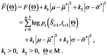 (28)
(28)
The variable metric steepest ascent method 1) - 7) is now applied to solve problem (24) when the (five variables) (log-)likelihood function  defined in (28) replaces the (log-)likelihood function
  defined in (22) starting from the initial guess:
 (29)
(29)
where the initial values  and
and  are estimated directly from the input data through (11) and, finally, the initial value
  is chosen as a rough estimate of the average amplitude of the spikes appearing in the input data. That is problem (24) is solved replacing
  with
with  starting from an initial guess that uses the results obtained in the preliminary step of the optimization procedure and tries to exploit the data using the “physical” meaning of the model parameters.
These ad hoc steps used to reformulate problem (24), when applied to the analysis of synthetic data, lead to a substantial improvement in the accuracy of the estimates of the model parameters obtained when compared to the estimates obtained solving directly (22), (24) and to a great saving in the computational cost of solving the calibration problem. This reformulation of problem (24) is used to analyze the data considered in Section 4.
As a byproduct of the solution of the calibration problem we obtain a technique to forecast forward asset prices. Let us consider a filtering problem. We assume that the vector  solution of the calibration problem associated to the data
 is known. From the knowledge of
  at time
  we can forecast the forward asset prices with delivery period
  deep in the future and delivery time
  as follows:
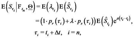 (30)
(30)
where  denotes the expected value of
 .
.
In the numerical experiments presented in Section 4 we use the following approximation:
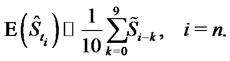 (31)
(31)
Note that using formula (31) we have implicitly assumed . In fact in the data time series considered in Section 4 the average in time of the (spiky) observations appearing in (31) gives a better approximation of the “spatial” average
  of the price without spikes than the individual observation
  made at time
  of the spiky price. However the average in time of the observations approximates the “spatial” average only if short time periods are used. This is the reason why we limit the mean contained in (31) to the data corresponding to ten consecutive observation times, that is corresponding to a period of ten days when we process daily data as done in Section 4. Note that in (31) an average of spiky prices is used to approximate the expected value of non spiky prices.
4. Numerical Results
The first numerical experiment presented consists in solving the calibration problem discussed in Section 3 using synthetic data. This experiment does the analysis of a time series of daily data of the spiky asset price during a period of two years. The time series studied is made of 730 daily data of the spiky asset prices, that is the prices  at time
 ,
,  These data have been obtained computing one trajectory of the stochastic dynamical system used to model spiky asset prices defined in Section 2 looking at the computed trajectory at time
 ,
,  with
with 
 where we have chosen
  and
and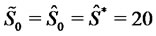 . We choose the vector
  that specifies the model used to generate the data equal to
  in the first year of data (i.e. when
 ,
, ), and equal to
 in the second year of data (i.e. when
 ). The data are generated using as initial value of the second year the last datum of the first year. The synthetic data generated in this way are shown in Figure 1. These data are spiky data and the fact that the first year of data is generated using a different choice of
  than the choice made in the second year of data can be seen simply looking at Figure 1.
We solve problem (24) with the ad hoc procedure described in Section 3 using the data associated to a time window made of 365 consecutive observation times, that is 365 days (one year), and we move this window across the two years of data discarding the datum corresponding to the first observation time of the window and inserting the datum corresponding to the next observation time after the window. Note that numerical experiments suggest that it is necessary to take a large window of observations to obtain a good estimate the parameters 
 and
and . The calibration problem is solved for each choice of the data time window applying the procedure described in Section 3, that is it is solved 365 times. The 365 vectors
  constructed in this way are compared to the two choices of the model parameters
  used to generate the data. Moreover the time when
  changes from being
  to being
  is reconstructed.
To represent the 365 vectors obtained solving the calibration problem in correspondence to the 365 data time windows considered, we associate to each reconstructed vector  a point on a straight line (see Figure 2). Let us explain how this correspondence is established. We first represent the vectors
  and
and  that generate the data as two points on the straight line mentioned above having a distance proportional to
  measured in
  units, where
Figure 2. Reconstruction of the parameter vectors  and
and 
 and
and
 . We choose the origin of the straight line to be the mid point of the segment that joins
  and
and  In Figure 2 the diamond represents the vector
  and the square represents the vector
  The unit length is
  The vectors (points) solution of the 365 calibration problems are represented as (green or red) stars. A point
  is plotted around
  when the quantity
  is smaller than the quantity
 , otherwise the point
  is plotted around
The distance of the point  from
from  when
when  is plotted around
  (or from
  when
when  is plotted around
 ) is
) is  measured in
  units (or
 measured in
  units). The point
  plotted around
  is plotted to the right or to the left of
  according to the sign of the second component of
  (negative second component of
  is plotted to the left of
 ). Remind that the second component of
  is the volatility coefficient
  A similar statement holds for the points plotted around
  The results obtained in this experiment are shown in Figure 2. In this figure the green stars represent the solutions of the calibration problems associated to the first 183 data time windows, that is the first “half” of data time windows, while the red stars represent those associated to the second “half” of the data time windows (that is the second 182 time windows). Figure 2 shows that the points (vectors) obtained solving the calibration problems are concentrated on two disjoint segments one to the left and one to the right of the origin and that they form two disjoint clusters around
  and
and  That is, the solution of the 365 calibration problems corresponding to the 365 time windows described previously shows that two sets of parameters seems to generate the data studied. This is really the case. Moreover, as expected, the points of the cluster around
  are in majority red stars, that is they are in majority the points obtained by the analysis of data time windows containing a majority of observations made in the second year (the second “half” of the data time windows), and a similar statement holds for the points of the cluster around
  (in majority green stars).
The second numerical experiment is performed using real data. The real data studied are electric power price data taken from the UK electricity market. These data are “spiky” asset prices. The data time series studied is made of the observation times  (days), and of the spiky asset price
  observed at time
 , where
  is the daily electric power spot price (GBP/MWh), named Day-Ahead price,
  Excluding week-end days and holidays this data time series corresponds to more than 5 years of daily observations going from January 5, 2004 to July 10, 2009. Remind that GBP means Great Britain Pound and that MWh means Mega-Watt/hour.
Moreover the data time series studied in correspondence of each spot price contains a series of forward prices associated to it for a variety of delivery periods. These prices include: forward price 1 month deep in the future (Month-Ahead price), forward price 3 months deep in the future (Quarter-Ahead price), forward price 4 months deep in the future (Season-Ahead price), forward price 1 year deep in the future (One Year-Ahead price). These forward prices are observed each day  and the forward prices observed at time
  are associated to the spot price
 The spot and the forward prices contained in the data time series mentioned above are shown in Figure 3.
The observed electric power prices generate data time series with a complicated structure. The stochastic dynamical system studied in this paper does not pretend to fully describe the properties of the electric power prices. Indeed it is able to model only one property of these prices: the presence of spikes. In addition the electricity prices have many other properties, for example, they are mean reverting and have well defined periodicity, that is they have diurnal, weekly and seasonal cycles. A lot of specific models incorporating (some of) these features are discussed in the literature, see for example [10].
Let us begin performing the analysis of the data using the model introduced in Section 2. The first question to answer is: the model for spiky prices presented in Section 2 is an adequate model to analyze the time series of the spot prices? We answer to this question analyzing the relationship between the data and the model parameters established through the solution of the calibration problem. Let us begin showing that the relation between the data and the model parameters established through the calibration problem is a stable relationship. We proceed as follows. We have more than 5 years of daily observations. We apply the calibration procedure to the data corresponding to a window of 257 consecutive observation times. Note that 257 is approximately the number of working days contained in a year and remind that we have data only in the working days. We move this window through the data time series discarding the datum corresponding to the first observation time of the window and adding the datum corresponding to the next observation time after the window. In this way we have 1396 − 257 = 1139 data windows and for each one of these data windows we solve the corresponding calibration problem. The calibration problems are solved using the optimization procedure (including the ad hoc steps) described in Section 3. The reconstructions of the parameters obtained
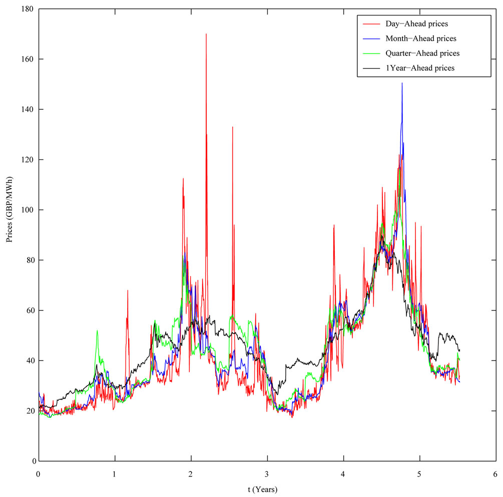
Figure 3. The UK electric power price data.
moving the window along the data are shown in Figures 4 and 5. In Figures 4 and 5 the abscissa represents the data windows used to reconstruct the model parameters numbered in ascending order according to the order in time of the first day of the window. Figures 4 and 5 show that the model parameters, with the exception of  are approximately constant functions of the data window. The parameter
  reconstructed shown in Figure 5 is a piecewise constant function. These findings support the idea that the model and the formulation of the calibration problem presented respectively in Sections 2 and 3 are adequate to interpret the data. In fact they establish a stable relationship between the data and the model parameters as shown in Figures 4 and 5.
In the analysis of the real data time series the second question to answer is: the solution of the calibration problem and the tracking procedure introduced in Section 3 can be used to forecast forward prices? To answer this question we compare the observed and the forecasted forward prices. We apply the calibration procedure to a data window made of the first three years of consecutive observations of the spot price taken from the data time series shown in Figure 3 and we use the solution of the calibration problem found and formulae (30), (31) to
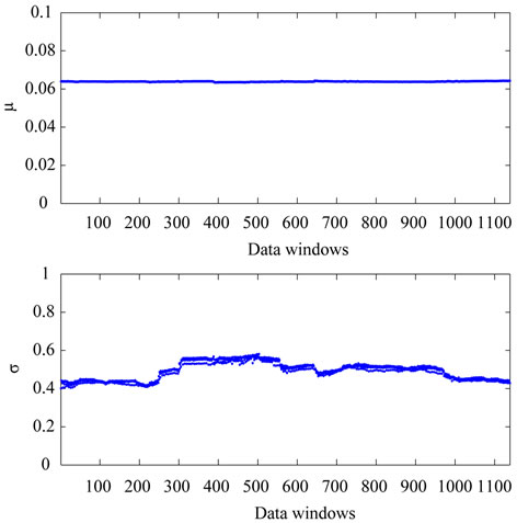
Figure 4. Reconstruction of the parameters of the BlackScholes model: μ, σ.
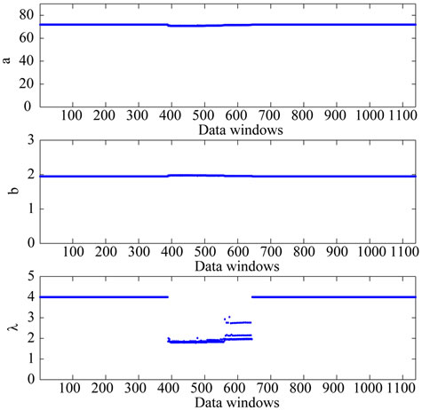
Figure 5. Reconstruction of the parameters used to model the spikes: a, b, λ.
calculate the forecasted forward prices associated to the spot prices of the data time series not included in the data window mentioned above used in the calibration problem. In Figures 6-8 the forward electric power prices forecasted are shown and compared to the observed forward electric power prices. In Figures 6-8 the abscissa is the day of the spot price associated to the forward prices computed. The abscissa of Figures 6-8 is coherent with the abscissa of Figure 3. Table 1 summarizes quantitatively the results shown in Figures 6-8 and gives the
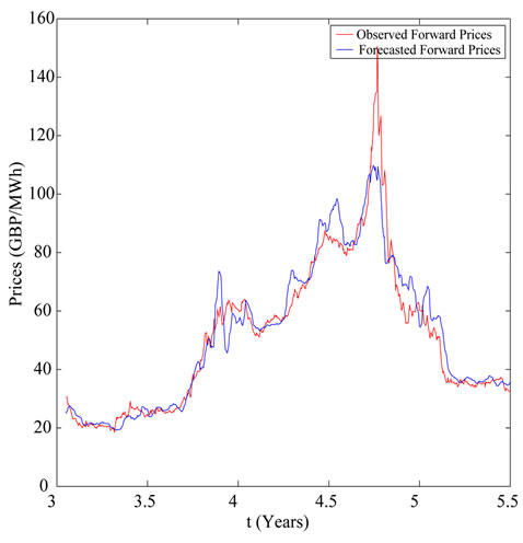
Figure 6. Month-ahead prices.
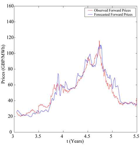
Figure 7. Quarter-ahead prices.
average relative error  committed using the forecasted forward prices, that is the average relative error committed approximating the observed forward prices with the forecasted forward prices. Table 1 and Figures 6-8 show the high quality of the forecasted forward prices answering the second question posed about the analysis of the data time series in the affirmative.
We can conclude that the data analysis presented shows that the model introduced to describe spiky prices, the formulation of the calibration problem and its numerical
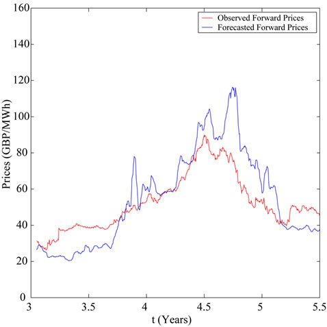
Figure 8. One year-ahead prices.
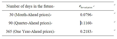
Table 1. Average relative errors of the forecasted forward electric power prices when compared to the observed forward prices.
solution presented in this paper have the potential of being tools of practical value in the analysis of data time series of spiky prices.
REFERENCES
- V. A. Kholodnyi, “Valuation and Hedging of European Contingent Claims on Power with Spikes: A Non-Markovian Approach,” Journal of Engineering Mathematics, Vol. 49, No. 3, 2004, pp. 233-252. doi:10.1023/B:ENGI.0000031203.43548.b6
- V. A. Kholodnyi, “The Non-Markovian Approach to the Valuation and Hedging of European Contingent Claims on Power with Scaling Spikes,” Nonlinear Analysis: Hybrid Systems, Vol. 2, No. 2, 2008, pp. 285-304. doi:10.1016/j.nahs.2006.05.002
- F. Mariani, G. Pacelli and F. Zirilli, “Maximum Likelihood Estimation of the Heston Stochastic Volatility Model Using Asset and Option Prices: An Application of Nonlinear Filtering Theory,” Optimization Letters, Vol. 2, No. 2, 2008, pp. 177-222. doi:10.1007/s11590-007-0052-7
- L. Fatone, F. Mariani, M. C. Recchioni and F. Zirilli, “Maximum Likelihood Estimation of the Parameters of a System of Stochastic Differential Equations that Models the Returns of the Index of Some Classes of Hedge Funds,” Journal of Inverse and Ill Posed Problems, Vol. 15, No. 5, 2007, pp. 493-526. doi:10.1515/jiip.2007.028
- L. Fatone, F. Mariani, M. C. Recchioni and F. Zirilli, “The Calibration of the Heston Stochastic Volatility Model Using Filtering and Maximum Likelihood Methods,” G. S. Ladde, N. G. Medhin, C. Peng and M. Sambandham, Eds., Proceedings of Dynamic Systems and Applications, Dynamic Publishers, Atlanta, Vol. 5, 2008, pp. 170-181.
- L. Fatone, F. Mariani, M. C. Recchioni and F. Zirilli, “Calibration of a Multiscale Stochastic Volatility Model Using European Option Prices,” Mathematical Methods in Ecomics and Finance, Vol. 3, No. 1, 2008, pp. 49-61.
- L. Fatone, F. Mariani, M. C. Recchioni and F. Zirilli, “An Explicitly Solvable Multi-Scale Stochastic Volatility Model: Option Pricing and Calibration,” Journal of Futures Markets, Vol. 29, No. 9, 2009, pp. 862-893. doi:10.1002/fut.20390
- L. Fatone, F. Mariani, M. C. Recchioni and F. Zirilli, “The Analysis of Real Data Using a Multiscale Stochastic Volatility Model,” European Financial Management, 2012, in press.
- P. Capelli, F. Mariani, M. C. Recchioni, F. Spinelli and F. Zirilli, “Determining a Stable Relationship between Hedge Fund Index HFRI-Equity and S&P 500 Behaviour, Using Filtering and Maximum Likelihood,” Inverse Problems in Science and Engineering, Vol. 18, No. 1, 2010, pp. 93-109.
- C. R. Knittel and M. R. Roberts, “An Empirical Examination of Restructured Electricity Prices,” Energy Economics, Vol. 27, No. 5, 2005, pp. 791-817. doi:10.1016/j.eneco.2004.11.005
- J. H. Hull, “Options, Futures, and Other Derivatives,” 7th Edition, Pearson Prentice Hall, London, 2008.
NOTES
*The research reported in this paper is partially supported by MUR— Ministero Università e Ricerca (Roma, Italy), 40%, 2007, under grant: “The impact of population ageing on financial markets, intermediaries and financial stability”. The support and sponsorship of MUR are gratefully acknowledged.
#The numerical experience reported in this paper has been obtained using the computing grid of ENEA (Roma, Italy). The support and sponsorship of ENEA are gratefully acknowledged.