Open Journal of Marine Science
Vol. 2 No. 3 (2012) , Article ID: 21415 , 5 pages DOI:10.4236/ojms.2012.23011
Potential Ecosystem Level Effects of a Shrimp Trawling Fishery in La Paz Bay, Mexico
Centro Interdisciplinario de Ciencias Marinas del IPN, Apartado Postal, La Paz, México
Email: salcidog@gmail.com, {pdelmontel, *farregui, vescalon }@ipn.mx
Received March 10, 2012; revised April 12, 2012; accepted May 15, 2012
Keywords: Gulf of California; Shrimp Trawling; Ecosystem Impact
ABSTRACT
The shrimp trawling fishery is the most important one in Mexico in value terms and given its putative environmental, societal and economical implications, it is also the most difficult to manage. Although this fishery was restricted from national bays and estuaries since the 1970’s, local fisheries cooperatives recently claimed access to shrimp stocks within La Paz Bay by using an artisanal fleet and a low impact trawling net. This study is aiming at simulating some ecosystem level effects of such a potential fishing effort release. We explored the response of three ecosystem indicators under two different exploitation scenarios: 30% and 80% of shrimp biomass removal. The indicators were: relative ecosystem biomass distribution as function of trophic level, trophic replacement and interaction strength, all computed from the outputs of a mass balance dynamic model (Ecopath with Ecosim) of this ecosystem. Our results suggest that moderate fishing scenario (30%) would not cause major changes in either indicator whilst the scenario of strong fishing pressure (80%) seems to increase not only the fish resources variability at the population level but also the variability of the overall biomass, hence potentially reducing ecosystem stability.
1. Introduction
In 2006, the economic income of the shrimp fishery in the Gulf of California was in excess of $411 million, ranking the first place as for the total value of marine resources. In the Mexican Pacific, roughly 1500 vessels target marine shrimp stocks; more than 70% of this fleet operates in Sonora, Sinaloa, Baja California and Baja California Sur [1] producing near 30,000 direct jobs. The gulf also hosts 90% of the shrimp farming industry, developed mostly during the 90’s and currently producing around 40% of the national shrimp tonnage [2].
Although the shrimp fishery is the most lucrative one in Mexico, it is also the most difficult to manage. The fact that this activity has been a cornerstone for the regional development during the last 50 years, counteracts with the environmental effects attributable to the fleet operation (habitat loss, fishing mortality of non-target animal and plant species), the recent decreasing trend of the catch per unit of effort, overcapitalization of the industry, federal subsidies and the concomitant societal and economic impacts. In light of this situation the academic, governmental and social sectors are deeply concerned over the long term ecological sustainability of the Mexican shrimp fishery. As a part of the government’s response to this problem, since 1993 a portion of Sonora and Sinaloa’s shrimp trawling fleet that had operated on sandy bottoms in La Paz Bay, was officially banned [3].
However in 2005, local fishing cooperatives claimed access to shrimp stocks within the bay (Figure 1) and asked the federal and state governments to evaluate the possibility of initiating a small-scale shrimp-trawling fishery. During that time, basic scientific information was required for estimating the available shrimp biomass and allowable fishing rates. Even when Mexican laws prohibit trawling fishing within bays and estuaries, such a request was based on the use of a low-impact fishing net, developed by the National Fisheries Institute, locally known as “Magdalena 1”, that operates in Magdalena Bay on the Pacific coast of the southern Baja California Peninsula. However, given the experience gained from the Incofish project (www.incofish.org) concerning the ecosystem level impacts of by-catch mortality associated with shrimp trawling, we were asked to carry out an evaluation of the potential effects of this fishery opening.
This study is aiming to address some potential ecosystem level effects if fishing effort of artisanal shrimp trawling was unleashed in La Paz Bay, by applying three ecological indicators: relative ecosystem biomass distribution
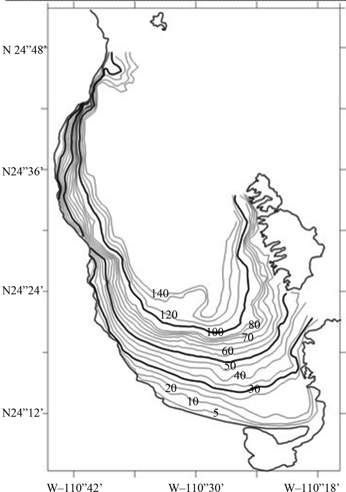
Figure 1. Study area showing bathymetry (increasing step is 5 meters).
as function of trophic level (RBD), trophic replacement (TR) and interaction strength (IS) computed from the outputs of a mass balance dynamic model Ecopath with Eocsim [4]).
2. Materials and Methods
The present study is based on an Ecopath mass balance model of La Paz Bay [5]. Previous models were constructed emphasizing artisanal finfish fisheries, but the model used for this study considers the addition of an artisanal shrimp trawling fleet and the associated bycatch. In this model, 25 out of 48 functional groups appear as by-catch and of those 14 species also appear as commercial catch in other fisheries. Since trawling activities are prohibited within the bay, the functional groups in the model were defined by considering the by-catch caught by artisanal shrimp boats, the target species exploited by commercial fleets as well as charismatic species such as marine mammals and aquatic birds. Main parameters per group are shown in Table 1.
Time simulations were made by using Ecopath with Ecosim (EwE) software, which provides a tropho-dynamic
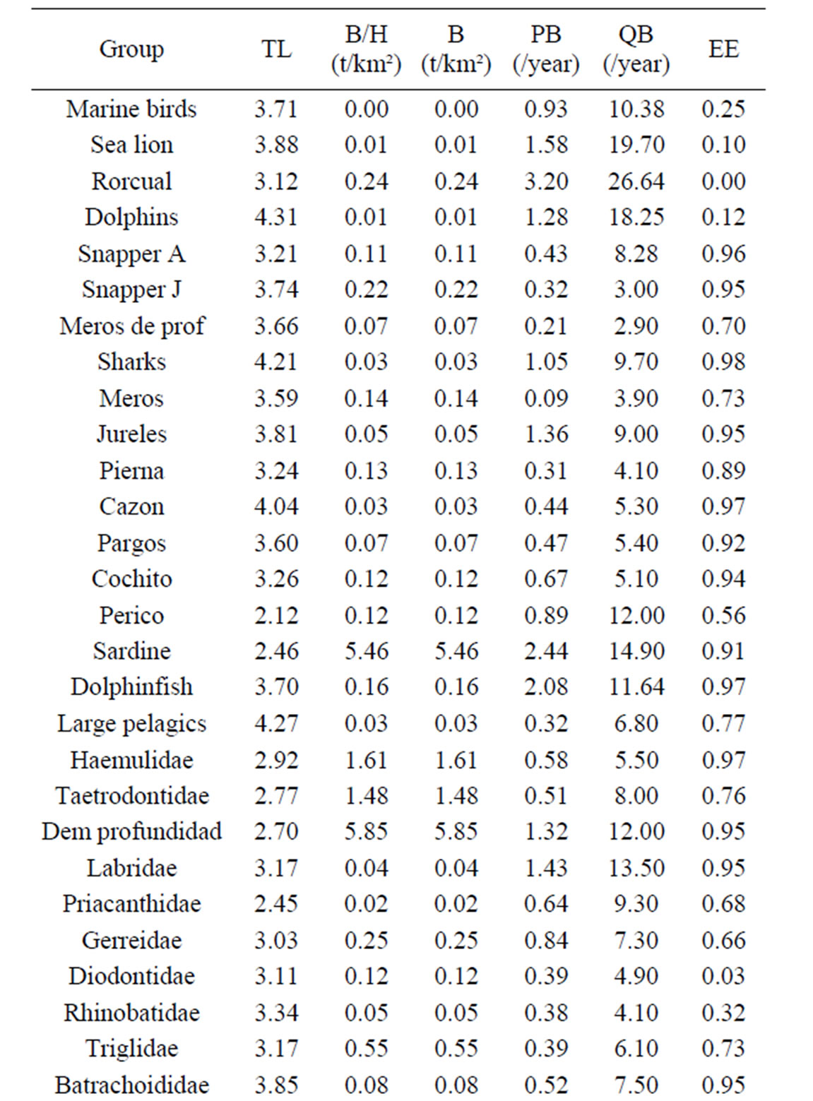
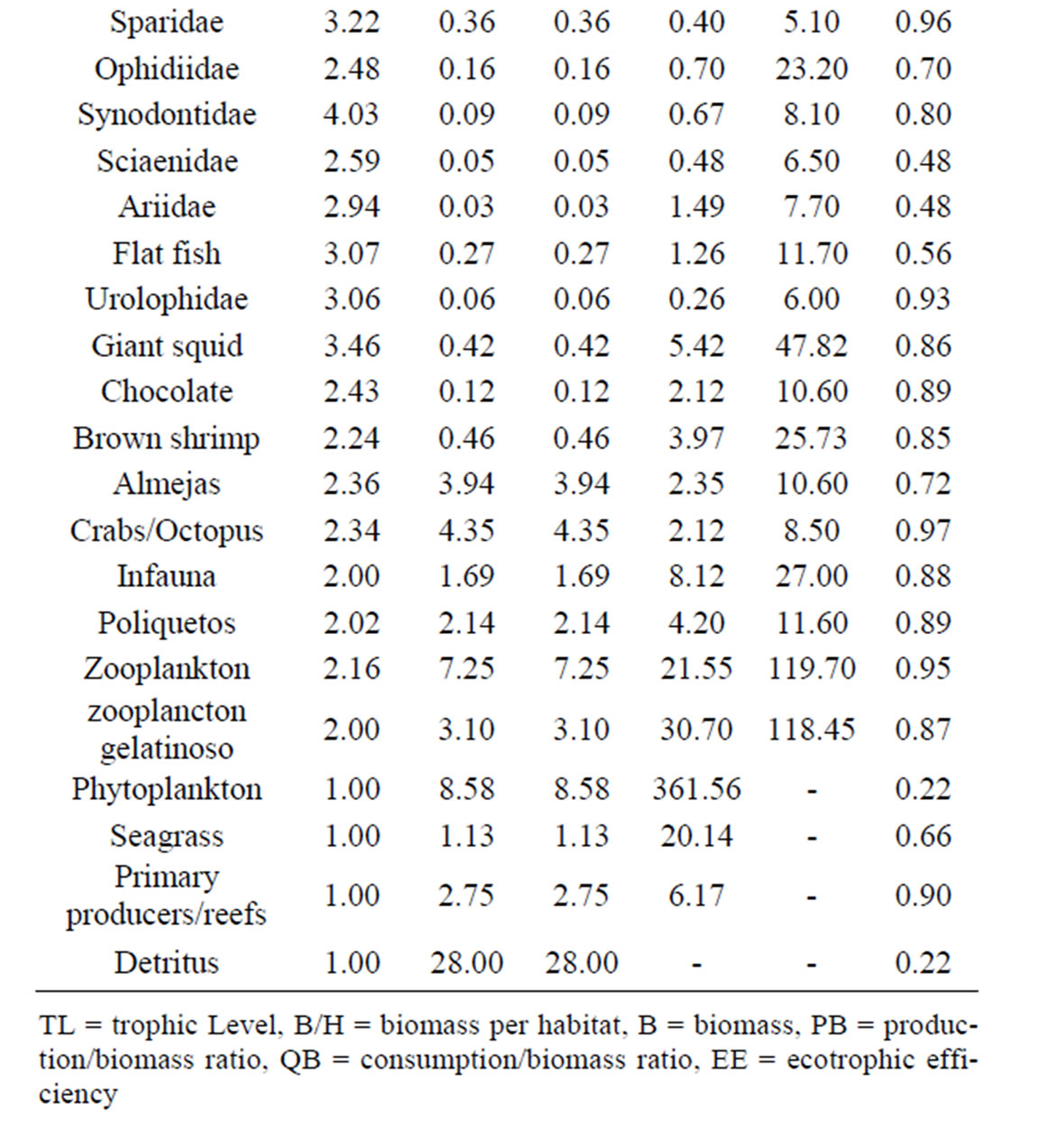
Table 1. Main parameters per functional group in the ecosystem of La Paz Bay (Arreguín-Sánchez et al., 2007).
simulation with ecosystem level considerations. EwE, through a system of differential equations, estimates energy flow rates among groups as a function of harvest rates and biomass changes through time for all functional groups in the model [6-8]. The instantaneous (Ecopath) mass balance model is defined by the following Equation:
where Bi and Bj are biomasses (the latter pertaining to j, the consumers of i), P/B their production/biomass ratio, equivalent to total mortality rate, EEi the fraction of production that is consumed within, or caught from the system, Yi is the fisheries catch (Y = FB; F is fishing mortality rate), Q/Bj the food consumption per unit biomass of j, and DCji the contribution of prey i to the diet of predator j.
The dynamic form of the model (Ecosim) is defined as:
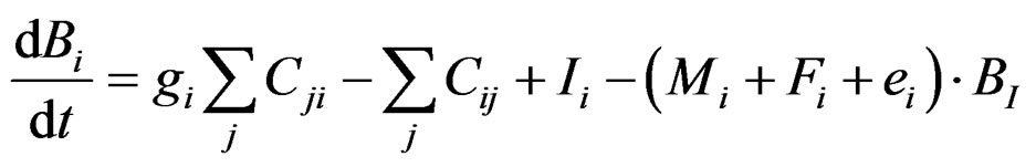
where dB/dt is rate of change in biomass, g is growth efficiency, F is fishing mortality rate, M is natural mortality rate (excluding predation), e is emigration rate, I is immigration rate, and Cij (Cji) is the consumption rate of type i (j) biomass by type j (i) organisms.
We explored two different fishing scenarios affecting the group denominated as “brown shrimp” (Farfantepeneaus californiensis), and their ecosystem level effects through three indicators: relative ecosystem biomass distribution by trophic level (RBD), trophic replacement (TR) [9] and interaction strength (IS) [9]. Fishing mortality patterns were defined according to the exploitation rate Equation (ER) [10]:
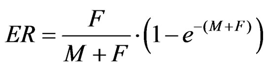
ER is proportional to the total stock biomass and can have values from 0 to 1, being 1 the exploitation rate equivalent to extracting the whole population. For each ER value (at each simulation year) we iteratively estimated the correspondent fishing mortality. The first scenario was one of moderate fishing exerted on shrimp stock, beginning in year 20 such as at the end of the simulation ER = 0.30 (i.e. 30% of the virgin biomass is removed). The correspondent F values ranged from F = 0 up to F = 5. In the second scenario, one of stronger fishing intensity, the exploitation began at year cero and ended with an ER = 0.80. In this case F values ranged from F = 0 up to F = 15. For both scenarios the simulation time-frame was 70 years.
Trophic replacement TR indicator quantifies the trophic replacement of a species that is removed from a system or drastically reduced in biomass (e.g. collapsed through overfishing) by other species or group in the system. It quantifies the extent to which trophic niche replacement occurs following a collapse of, or increases in, a target stock. The TR indicator is calculated for each group j (and year) belonging to the set of groups (K) that show a change in biomass of the opposite sign to that of the target group i (e.g. if target group i collapses, K is a group undergoing an increase following the collapse of group i:
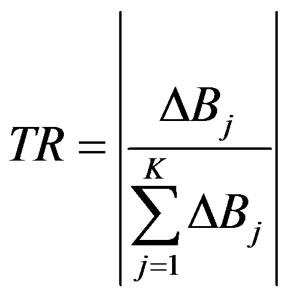
where ΔB is the change in biomass of any group between consecutive years. The indicator ranges between 0 (no replacement) and 1 (total replacement).
IS indicator assumes that a change in biomass of a strong interactor causes large changes in the biomass of other groups. The relative change in the biomass of a species or functional group is expressed as a proportion of the sum of the relative changes of all groups in the system:
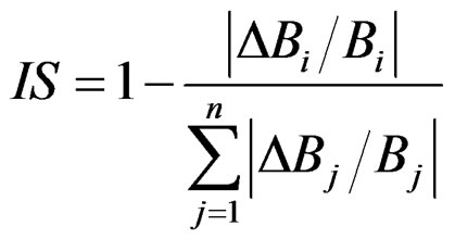
where B is biomass in year 0, i is the group being tested, j is another functional group in the ecosystem, ΔB is the change in biomass of a group and n is the total number of groups in the model. Values for the indicator lie between 1 and 0, with large values indicating that species (or group) i has a stronger impact on other groups than species with smaller values. IS and TR were derived from the trophic model outputs for each group and year of simulation.
After the simulation, biomass data were standardized considering the highest value of each individual group at each year as the unit (1). In this way, differences in magnitude of biomass among groups become proportional (RBD). Groups in all cases were sorted by trophic level. Resulting matrices (groups/species sorted by trophic level in the ordinate, simulation years in the abscissa and indices values in the vertical axis) were plotted as surface diagrams.
3. Results
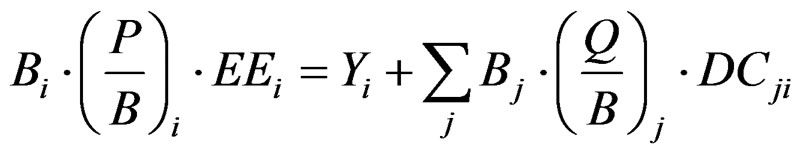
Results are shown in Figure 2. The first exploitation scenario reveals no apparent effect on ecosystem properties (Figures 2(a), (c) and (e)). There are three discernible stages in the RBD (Figure 2(a)): the first one is an initial stability period, from year cero to roughly year 32 (10 years after the fishing pressure began). The second is a transition period, starting at year 35 and ending at year 45, in which biomasses begin to invert their original trend. Last stage, ranging from year 50 onwards, represents the opposite of stage one; the RDB, however, maintains a constant structure during this period. A similar pattern, although less variable, is observed in TR and IS (Figures 2(c) and (e)).
The second scenario, as it involves extracting 80% of the shrimp population biomass, notably modifies the behavior of all indicators over time, particularly RBD. Analyzing the RBD in different time windows, it is evident that the degree of variation is constantly increasing over time until a similar pattern to that of the last stage of the biomass distribution in the first scenario is reached, though exacerbated and of much less duration (10 years); i.e. small (high) values in scenario 1 are smaller (higher) in scenario 2. The IS index shows comparable changes between the two scenarios. In the first one, the TR level is considerable high in all functional groups, and in the second one it displays higher variation but of lesser intensity.
4. Discussion
Previous population and ecosystem dynamic models applied to the shrimp fishery in La Paz Bay indicate that if trawling activity operates without any depth restriction, then extracting 38% of the whole population represents a target reference point. At this level of extraction, ecosystem impacts would not be significant in terms of the trophic structure and the mean trophic level of the catch. If the fishery is restricted to depths in excess of 40 m, then the fraction of the population that can be extracted increases to 50% without significantly affecting those ecosystem indices (F. Arreguín-Sánchez, unpublished data).
These results are compatible with ours. As the first scenario indicates, a moderate fishing pressure causes slight changes in ecosystem biomass and biomass stability, even after removing 30% of shrimp biomass. Likewise, it was found that trawling fishery in La Paz Bay positively impacts shrimp populations [11] since, at the same time, reduces their predators. It seems that predator removal causes a stronger positive impact on shrimps that does the negative impact of fishing, which is also coherent with what we found. In the first scenario, the evolution of the relative biomass around the trophic level of the brown shrimp (2.5) along the simulation period shows a slight decline, concomitant with a biomass reduction in higher trophic levels (shrimp predators). Under a heavy fishing condition, though, both, shrimp and predators biomasses sharply decline by year 40 (Figures 2(a) and (b)).
Other indicators show that brown shrimp in La Paz Bay naturally have low TR and IS values. Once fishing pressure starts affecting shrimp populations, both indicators increase (Figures 2(c) and (d)). This suggests that fishing pressure has small effects on either indicator; perhaps shrimps and groupers display the more noticeable changes (Figures 2(c), (e) and (f)). In the case of shrimps, being trophic generalists they are more prone to be replaced by similar species. Furthermore, faunal assemblages in La Paz Bay may be sufficiently diverse as to allow a dynamic functional replacement of fish populations decimated by exploitation [12,13].
On the other hand, IS evolution suggests that brown shrimp, being a foraging species, has an important trophic role in the ecosystem, tightening the interaction with its many predators as it is increasingly fished down (Figure 2(f)). The IS also increases over time in the group of the puffers (Tetraodontidae, trophic level = 2.77; Figure 2(f)). The effect of fishing on this group is similar because they are among the most abundant fish extracted
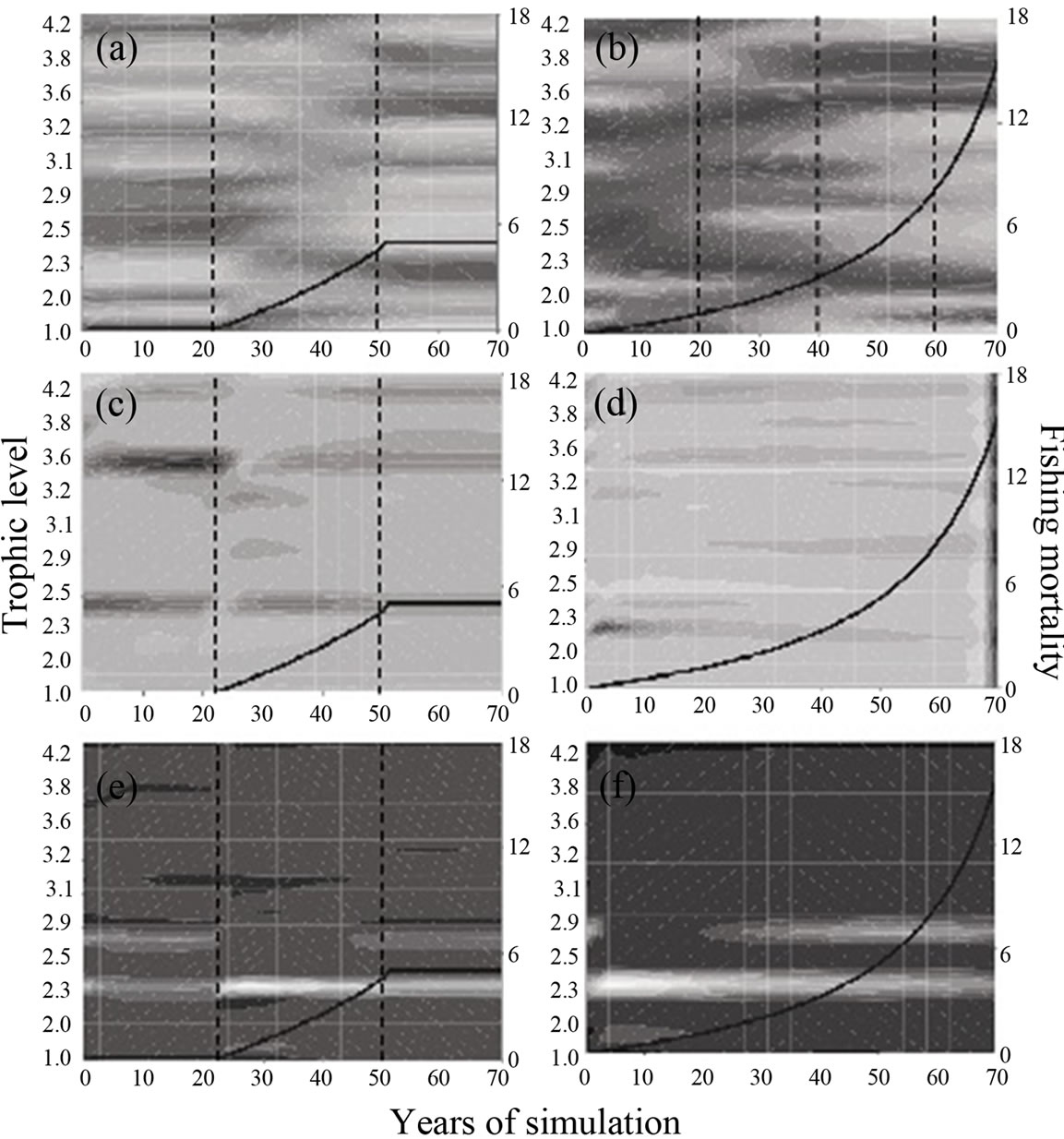
Figure 2. Evolution diagrams of biomass (B; (a) and (b)), trophic replacement index (TR; (c) and (d)) and interaction strength index (IS; (e) and (f)) derived from Ecosim dynamic simulation (70 years) of La Paz Bay ecosystem. Graphs on the left represent the response of B, TR and IS along all function al groups to an exploitation regime (whose maximum is) equivalent to extracting 30% of shrimp virgin biomass; exploitation begins at year 21 and reaches the plateau at year 50. Graphs on right hand depict the same but for a (continuous) exploitation regime equivalent to extracting 80% of shrimp virgin biomass. All plots are arranged by discrete trophic level (48 functional groups; left Y axis). Fishing mortality is shown in right Y axis. Vertical dotted lines indicate noticeable changes in the trend of variables. All scales are individually standardized between 0 (darker) and 1 (lighter).
by trawling gears in La Paz Bay, representing up to 90% of total catch, and are highly predated.
Moderate fishing scenario would not cause mayor changes in RBD, TR nor IS. The more noticeable modification is the biomass reversion across all trophic levels, although, without risking the ecosystem stability. Conversely, a scenario of strong fishing pressure seems to increase fish resources variability at the population level and, as suggested [14], also the variability of the overall ecosystem biomass. TR and IS indicators, in general, showed limited response to fishing intensity, indicating that such variables (though not necessarily the process that they represent) may be relatively insensitive to the effects of fishing.
Actual harvest rate of the trawling fishery on shrimp populations within La Paz Bay is negligible and even if it started at moderately exploitation levels (F £ 5) would cause no significant change in other fish stocks (i.e. ecologically sustainable). However, a heavy fishing regime has the potential of disrupting ecosystem stability and resilience. More research is needed in order to quantitatively delimitate critical ecosystem threshold levels between these two conditions.
5. Acknowledgements
LASG thanks PIFI-IPN Program and CONACyT schoolarships. Authors thank partial support received through projects SIP-IPN (20121172, 20121444) and SEPCONACyT (104974, as well as COFAA and EDI programs of the Instituto Politécnico Nacional (IPN).
REFERENCES
- SAGARPA, Anuario Estadístico de Pesca, “Secretaría de Agricultura, Ganadería, Desarrollo Rural, Pesca y Alimentación. Comisión Nacional de Acuacultura y Pesca,” México, 2012, p. 265. http://www.conapesca.sagarpa.gob.mx/wb/cona/cona_anuario_estadistico_de_pesca
- S. E. Lluch-Cota, E. A. Aragón-Noriega, F. ArreguínSánchez, D. Aurioles-Gamboa, J. J. Bautista-Romero, R. C. Brusca, R. Cervantes-Duarte, R. Cortés-Altamirano, P. Del-Monte-Luna, A. Esquivel-Herrera, G. Fernández, M. E. Hendrickx, S. Hernández-Vázquez, H. Herrera-Cervantes, M. Kahru, M. Lavín, D. Lluch-Belda, D. B. Lluch-Cota, J. López-Martínez, S. G. Marinone, M. O. Nevárez-Martínez, S. Ortega-García, E. Palacios-Castro, A. Parés-Sierra, G. Ponce-Díaz, M. Ramírez-Rodríguez, C. A. Salinas-Zavala, R. A. Schwartzlose and A. P. Sierra-Beltrán, “The Gulf of California: review of ecosystem status and sustainability challenges,” Progress in Oceanography, Vol. 73, No. 1, 2007, pp. 1-26. doi:10.1016/j.pocean.2007.01.013
- Diario Oficial de la Federación, “Norma Oficial Mexicana 002-PESC-1993 para ordenar el aprovechamiento de las especies de camarón en aguas de jurisdicción federal de los Estados Unidos Mexicanos,” Secretaría de Gobernación, Gobierno de México, 2012 http://www.conapesca.sagarpa.gob.mx/wb/cona/cona_cuadro_de_noms
- D. Pauly, V. Christensen and C. Walters, “Ecopath, Ecosim, and Ecospace as tools for Evaluating Ecosystem Impact of fisheries,” ICES Journal of Marine Science, Vol. 57, No. 3, pp. 697-706. doi:10.1006/jmsc.2000.0726
- F. Arreguín-Sánchez, P. del Monte-Luna, J. G. Díaz-Uribe, M. Gorostieta, E. A. Chávez and R. Ronzón-Rodríguez, “Trophic Model For the ecosystem of La Paz Bay, Southern Baja California Peninsula, Mexico,” Fisheries Centre Research Reports, Vol. 15, No. 6, 2007, pp. 134-160. http://www.fisheries.ubc.ca/publications/incofish-ecosystem-models-transiting-ecopath-ecospace
- C. Walters, V. Christensen and D. Pauly, “Structuring dynamic models of Exploited Ecosystems from trophic mass-balance assessments,” Reviews in Fish Biology and Fisheries, Vol. 7, No. 2, 1997, pp. 139-172. doi:10.1023/A:1018479526149
- C. J. Walters, J. F. Kitchell, V. Christensen and D. Pauly, “Representing Density Dependent Consequences of Life History Strategies in Aquatic Ecosystems: EcoSim II,” Ecosystems, Vol. 3, No. 1, 2000, pp. 70-83. doi:10.1007/s100210000011
- V. Christensen and C. J. Walters, “Ecopath with Ecosim: methods, capabilities and limitations,” Ecological Modelling, Vol. 172, No. 2-4, 2004, pp. 109-139. doi:10.1016/j.ecolmodel.2003.09.003
- L. J. Shannon and P. M. Cury, “Indicators quantifying Small Pelagic Fish Interactions: Application Using a trophic model of the southern Benguela ecosystem,” Ecological Indicators, Vol. 3, No. 4, 2004, pp. 305-321. doi:10.1016/j.ecolind.2003.11.008
- W. E. Ricker, “Computation and interpretation of biological statistics of Fish Populations,” Department of the Environment, Fisheries and Marine Service, 1975.
- J. G. Díaz-Uribe, “Estrategias de evaluación para el manejo de la pesquería artesanal del huachinango (Lutjanus peru) en el sur del Golfo de California,” Ph.D. Thesis, Centro de Investigaciones Biológicas del Noroeste, S.C, México, 2005.
- E. F. Balart, J. L. Castro-Aguirre and F. De LachicaBonilla, “Análisis comparativo de las comunidades ícticas de fondos blandos y someros de la Bahía de La Paz, BCS,” In: J. Urbán-Ramírez and M. R. Rodríguez, Eds., La Bahía de La Paz investigación y conservación, Universidad Autónoma de Baja California Sur, La Paz, 1997, pp. 177-188.
- J. L. Castro-Aguirre and E. F. Balart, “Contribución al conocimiento de la ictiofauna de fondos blandos y someros de la Ensenada de La Paz y Bahía de La Paz, BCS,” In: J. U. Ramírez and M. R. Rodríguez, Eds., La Bahía de La Paz investigación y conservación, Universidad Autónoma de Baja California Sur, La Paz, 1997, pp. 139-150.
- C. Minto, R. A. Myers and W. Blanchard, “Survival Vari- ability and Population Density in Fish Populations,” Na-ture, Vol. 452, 2008, pp. 344-347. doi:10.1038/nature06605