Open Journal of Psychiatry
Vol. 2 No. 3 (2012) , Article ID: 21318 , 16 pages DOI:10.4236/ojpsych.2012.23023
Evidence of impaired facial emotion recognition in mild Alzheimer’s disease: A mathematical approach and application
![]()
1Unité de Psychiatrie du Sujet Agé (UPSA), Centre Hospitalier de Valenciennes, Valenciennes, France
2Department of Psychiatry and Behavioral Sciences, College of Medicine, University of Oklahoma, Oklahoma City, USA
3Brussels, Belgium
4Institute of Psychological Sciences, Center of Neuroscience, Cognition and Systems, University of Louvain, Louvain la Neuve, Belgium
Email: *philippe.granato@gmail.com
Received 5 April 2012; revised 1 May 2012; accepted 10 May 2012
Keywords: emotion perception; measure; morphed facial expression; categorical perception; logistic function; MARIE; Alzheimer
ABSTRACT
Objectives: The first objective of this paper is to show the improved binary outcomes resulting from using MARIE as a diagnostic instrument that allows valid and reliable visual recognition of facial emotional expressions (VRFEE) in an objective and quantitative manner. The second objective is to demonstrate mathematical modeling of binary responses that allow the measurement of categorical dimension, sensitivity, camber, equilibrium points, transition thresholds, etc. The final objective is to illustrate the use of this test for 1) testing a homogeneous sample of healthy young participants; and 2) applying this method to a sample of 12 participants with early Alzheimer disease compared to a matched control sample of healthy elderly participants. Design: Transforming the binary outcomes of MARIE in mathematical variables (experiment 1), allowing verification of a disorder of VRFEE in early Alzheimer’s disease (experiment 2). Measures: Comparison of numerical variables and graphic representations of both samples. Results: The objective measurement of VRFEE is possible in a healthy population. The application of this methodology to a pathological population is also made possible. The results support the current literature. Conclusion: The combination of the mathematical method with the diagnostic instrument MARIE shows its power and ease of use in clinical practice and research. Its application in many clinical conditions and in clinical research can be useful for understanding brain function. This method improves 1) the inter-examiner comparison and standardizes the quantification of VRFEE for use by multiple researchers; 2) the followup of a sample over time; 3) the comparison of two or more samples. This method is already available in clinical work for refining the diagnosis of Alzheimer’s Disease (AD) in our department.
1. INTRODUCTION
Facial emotional expression is a nonverbal communication channel which precedes language. The development of computer technology allows a more precise study of emotional expression. Emotion is a signal that borrows various channels: voice, posture, gestures and facial expressions. Metaphorically speaking, it is expressed by a transmitter and sensed by a receiver. We propose to study only the receiving system. The central nervous system allows the visual recognition of facial emotional expression (VRFEE) controlled by the receiver system. A feature of this system is the categorical dimension and most current literature confirms this. Categorical perception (CP) seems to be a fundamental property of perception, as it simplifies and reduces the complexity of the to-be-processed percept generated by the stimuli [1-10]. Indeed, even when a stimulus can take an infinite number of values between a minimum and a maximum, only a small number of categories are perceived. For instance, while the wavelength of the visible light can vary continuously between ±390 and ±700 nm, only seven different color categories are seen by the human perceiver. Thus, CP shows that the relationship between the stimulus and the perception is not a linear function, but rather a threshold or sigmoidal one. Consequently, the demonstration of a sharp category boundary is a diagnostic sign of CP.
In experimental psychology, CP has been demonstrated and studied since influential reports on the discrimination of phonemes [9,11-17] and the perception of colors [2,18]. Thanks to the development of computers and image processing softwares, it is now possible to make a continuous transition between a minimum and a maximum value of multidimensional stimuli like faces. By implementing these morphing techniques, numerous recent publications have revealed CP of face gender [19,20] face identity [1,5,8,21-23] and emotional facial expressions [6,10,12,19,21-35]. The resulting graphs typically take the form of a sigmoidor threshold-like function. However, from such a non-normal function, it is not feasible to calculate the traditional parameters like means, standard deviations, or variances. As a consequence, quantitative comparisons of two or more distributions are not amenable to computation. Therefore, we need a technique such as the one proposed here to circumvent the theoretical impasse presented by statistical approach [24,30-33]. A similar approach was recently proposed by Huang et al. [35]. The purpose of our mathematical method was to make it measurable and explicit series of 0 and 1 whose expressions were sigmoidal graphics (for details, see [24,30-33]).
This presents two challenges: 1) to define adequate parameters of the distributions; and 2) to design adequate statistical methods for comparisons. The purpose of the present study is to offer a way to overcome the former challenge. To achieve this, we chose a mathematical approach because we wanted to benefit from the highlevel algorithms implemented in most computed algebra software packages. The second challenge will be addressed in future developments, when we will make use of statistical methods to compare results obtained from these mathematical tools.
It is worth noting that many statistical attempts are already reported in the literature [4,12-14,16,31,35-38] These studies often use the probit analysis [6,39-46] in the framework of the analysis of the psychometric function [4,15,17]. However, while this statistical approach is able to determine coefficients and likelihood of validity and reliability of a model, it cannot study important properties of the function: camber, equilibrium points, transition thresholds, and so on (see the method section), except the slope [17,31,40]. This is why a mathematical approach was preferred. This method is similar to the logistic regression which is a statistical technique that aims to produce a model to predict the values of a categorical variable, usually binary, from a series of continuous explanatory variables and/or binary variables.
The aim of this work was to develop this mathematical method from the results of a sample of healthy young adults (experiment 1), and then to compare a sample of elderly patients with early Alzheimer’s disease to a matched sample of elderly healthy participants (experiment 2).
2. GENERAL METHOD: STIMULI AND PROCEDURE
The method was identical in both experiments. Each subject underwent a set of trials of recognition of emotions displayed in a series of images of a poser’s face. The stimuli were prepared and displayed by means of MARIE, a computerized tool already described in detail elsewhere [24,30-33]. In short, the test is based on a morphing procedure that converts gradually an image A into an image B. The number of pixels of image A and image B vary inversely to the distance from A and B. We created nine emotional series (ES) consisting of two canonical emotions and 17 chimeras (morphs). The 19 emotional images of each ES were shown to each subject in a random order. The subject had to respond by clicking the right or left mouse button. Each response was converted into 0 or 1. The stimuli were morphs drawn from 27 pairs of original photographs from Ekman and Friesen (with permission [29]), each pair being made of two basic emotional expressions, labeled A and B in what follows, displayed by the poser (the blond girl), displaying seven expressions: fear, anger, disgust, happiness, neutrality, sadness and surprise. Nine pairs of emotions were selected: angry-afraid, angry-sad, happy-sad, and all combinations of the neutral with the remaining six expressions. The contribution of picture B in AB morphs was 0, 10%, 20%, 30%, 35%, 38%, 41%, 44%, 47%, 50%, 53%, 56%, 59%, 62%, 65%, 70%, 80%, 90% and 100%. Therefore, this led to an ES of 19 stimuli including the original photographs (figure 1) for each pair of expressions: a total of 9 pairs of expressions × 19 pictures = 171 stimuli. First, the order of the nine pairs of expressions was selected at random for each subject. Then, the 19 stimuli of each ES were shown in a random order, with the exception that the last two images were systematically the original, unmorphed photographs, to
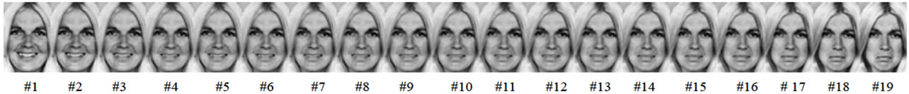
Figure 1. The happy/sad series for the Blond. The most left picture depicts the “pure” happy expression (A); The most right picture depicts the “pure” sad expression (B); The remaining 17 pictures are ranked by increasing values of the contribution of (B) to the picture.
avoid biases in the identification of expressions of the intermediate morphs.
For each stimulus (10 × 18 cm; viewing distance = 40 cm), the subject had to choose between two responses (A and B, e.g., angry and afraid) by pressing the left (A) or right (B) button of the mouse. The two corresponding labels of the expressions were displayed as prompts on the left and right side of the stimulus.
3. EXPERIMENT
3.1. Participants
The test was carried out with a sample of 30 healthy subjects (15 females) selected in accordance with a series of criteria in order to ensure that the sample was homogeneous (education level, handedness, gender). Subjects were 21 to 30 years of age, with normal or corrected-tonormal visual acuity. Subjects with detectable psychiatric and/or neurological disorders, and on medications, were excluded.
3.2. Pretest
As each image (n = 171) was shown only once to each subject, a pretest with five presentations was performed to check for the stability of responses. This control pretest involved 13 independent healthy subjects (6 females) between the ages of 29 and 41 (mean = 35; SD = 5), submitted to five repetitions of the 171 images. The criterion of stability of responses across repetitions was at least four identical responses out of five (80%). The grand mean was 93.1%. The criterion of 80% was reached for 160 out of 171 values. An agreement of 100% was observed for 36 of these 160 values. The remaining 11 values were tested against 80% by means of unilateral Student t tests. No value differed significantly from 80%. Consequently, it appeared that the single-trial procedure was sufficiently error-proof.
3.3. Data Analysis
The dependent variable was the number of subjects, out of 30, who chose expression B. Thus, choices pooled over subjects displayed the variable sensitivity existing within the group. Table 1 shows the results. These values were then analyzed to fit them to an adequately selected mathematical model. This model will furnish normative values for subsequent comparisons.
3.4. Results
3.4.1. Selecting the Model
Visual inspection clearly revealed that the data were distributed according to a symmetric sigmoid law (S-shaped curve). On the other hand, CP predicts a threshold or sigmoid relation between the proportion of subjects who chose expression B and the contribution of B in the picture shown (in percentage of pixels). This observation means that we were offered a choice between several possible mathematical models. We selected the logistic model [39,43] because it met four criteria. First, it had an adequate number of parameters (three: a, b and c) which can be computed in order to optimize the fitting process. Secondly, parameters were minimally covariant to minimize computation constraints. Thirdly, the number of
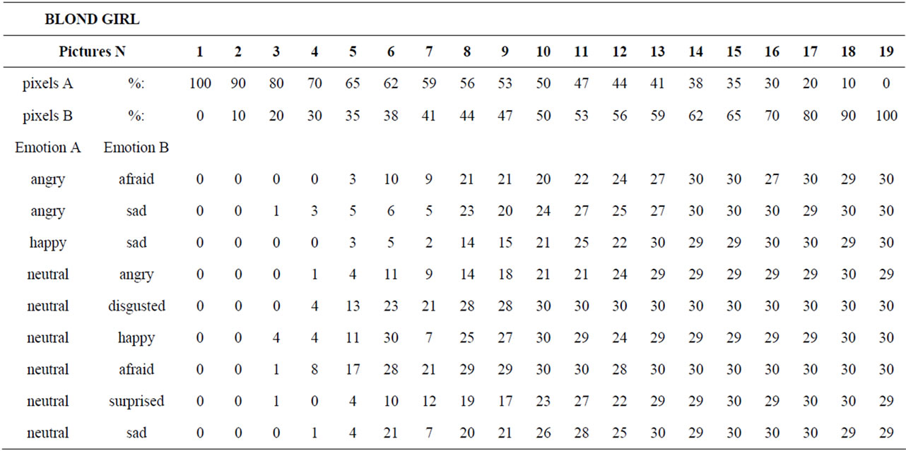
Table 1. Number of subjects, out of 30, who chose emotion B, for each picture of each series.
constants was small (two: 1 and the Neper’s constant e) without affecting the flexibility of the logistic model. And fourthly, the model could have symbolic (as opposed to numeric) solutions to compute derivatives and integrals.
3.4.2. Rebuilding the Logistic Model
Putting together the logistic model, we started by selecting a simple damping factor f(z) having the form of an inverse exponential function which reaches value 1 when z tends towards −∞ and value 0 when z tends towards +∞: f(z) = 1/(1 + ecz). Combining the damping factor with an exponential function, ecz, we get f(z) = ecz·1/(1 + ecz) = ecz/(1 + ecz) = 1/(1 + e−cz) which is the formula of the logistic model. In this formula, c parameter is inherited from the ordinary differential equation, initially developed to study population growth, and represents the initial growth rate. The simple logistic model lacks the flexibility that we needed to fit data that have a potential to vary substantially from one experimental session to another. Indeed, some emotional pairs are more difficult to perceive than others. Consequently, when recognition of expression B becomes difficult, the graph shifts to the right of the Cartesian system. So, to provide this essential flexibility, we added an extra location parameter (b) as a factor of the exponential. For ease of analyzing the graphs, we also added a scale parameter (a) to extend the scale of the ordinate axis to 100(%). Finally, our model became y = f(x) = a/(1 + b·e−cx) where “a” is the scale parameter, “b” the location parameter, and “c” the slope parameter. “y” is the percentage of responses B predicted by the model, and “x” the percentage of pixels of B in the morph. In other words, to obtain a, b and c we needed just two numbers for each ES: the percentage of responses B and the percentage of pixels B.
3.4.3. Assessing a, b and c: Logistic Regression
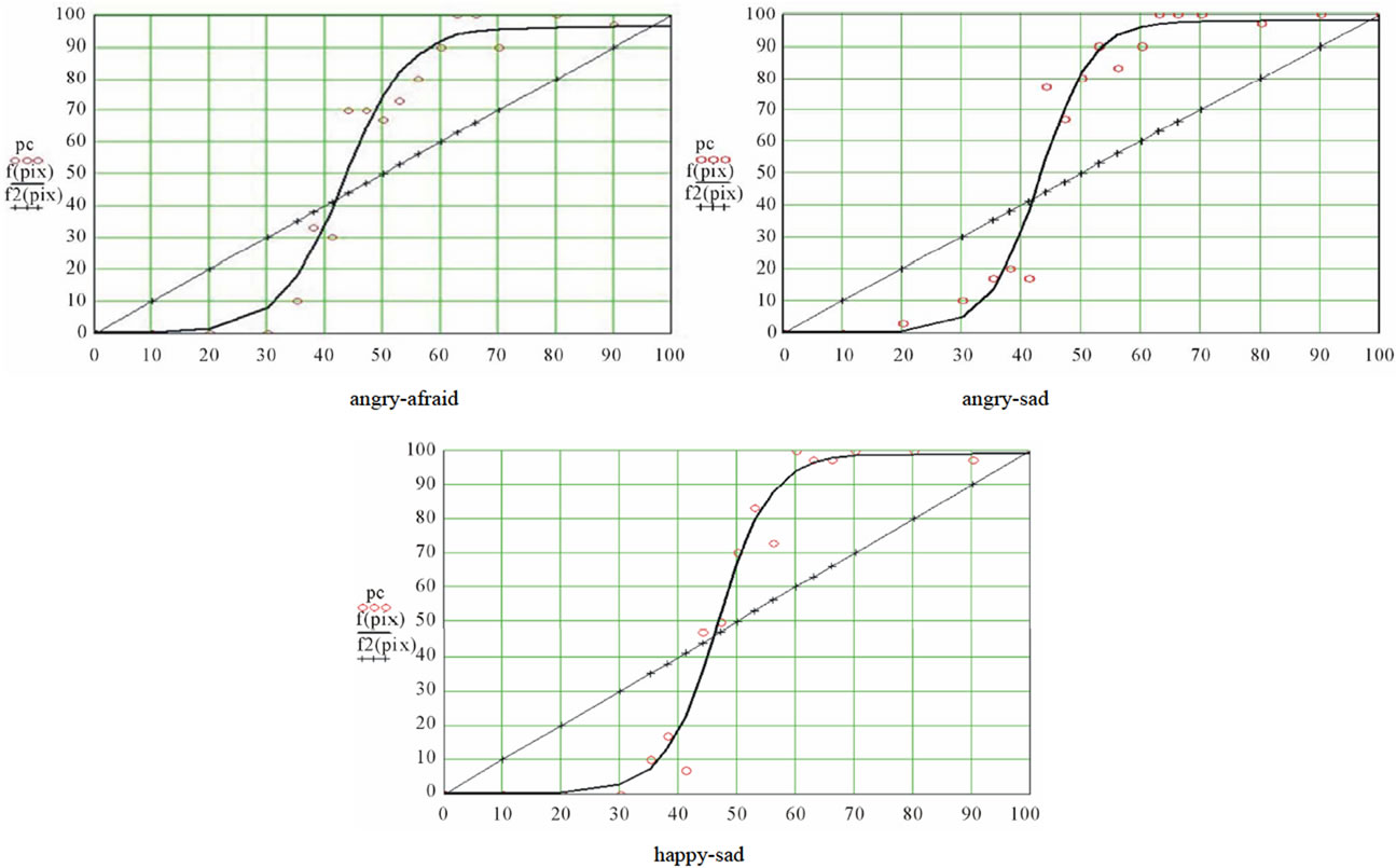
Logistic regression is an iterative process whereby different values of the parameters are tested at each iteration interval against a merit function, until this function reaches a stable minimum. Indeed, the merit function measures the agreement between observed data and the data provided by a fitting model for a particular selection of parameters; as a rule, the merit function is small when agreement is good. We selected the Levenberg-Marquardt algorithm [39]. For more details about the underlying rationale of this method, see More et al. [47]. The Levenberg-Marquardt algorithm provided us with the values of the three parameters for each of the nine ES. Computation of the standard errors and the correlations between predicted values and observed data insured that the fits were of good quality. The resulting distributions were graphed, and a stimuli distribution line was added (projecting the abscissa axis on a diagonal straight line) for the purpose of illustrating the categorization phenomenon. This diagonal has equation y = x. figure 2 is an illustration of the resulting graphs.
3.4.4. Properties of the Curves
Thanks to the parameters, it was possible to compute several relevant properties of the curves (see figure 3). The maximal value of the first derivative supplied us with the highest slope (or camber) of the curve; this value was then transformed in degrees. The value of yi where the maximal slope was observed corresponds to the inflexion point of the curve, i.e., is to say, the point where the second derivative = 0. Coordinates of the inflexion point were computed by calculating the abscissa and the ordinate as a/2. The abscissa supplied us with the contribution of emotion B in the (virtual) picture for which the number of responses B would be 50%, and can be considered in comparison to the morph where the contribution of emotion B was 50%, i.e. where xi = 50. The lapsing rate, defined as 100 – a, was an indication of
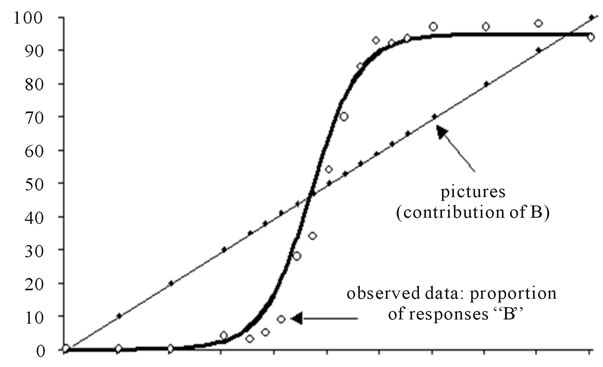
Figure 2. A typical curve resulting from the logistic regression. The circles represent the raw results and the bold curve adjustment function A stimuli distribution line was added (projecting the abscissa axis on a diagonal straight line) for the purpose of illustrating the categorization phenomenon. This diagonal has equation y = x.
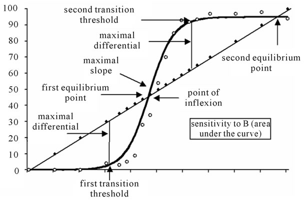
Figure 3. Properties of the curve. Demonstration of all parameter of graphical representation to the sigmoid function.
how much the group of subjects encountered difficulties in discriminating B from A. The sensitivity (to emotion B) was measured by the area under the sigmoid curve from 0 to 100% (the model’s integral) and showed the degree of sensitivity of the group to the emotion B. The binary data collected by means of MARIE precluded the use of traditional psychological measures of sensitivity such as d’ or A’. This is why the integral was considered as an index of sensitivity of the subjects to the emotion B in the AB bipolar ES (bipolar when A and B are two different emotional expressions, as in the pair angry-sad), and of the absolute sensitivity of the subjects to the expression B in unipolar ES (unipolar when A is the neutral expression [22] as in the pair neutral-sad). The transition thresholds were points of the curve where the ratio between the percentage of responses B and the percentage of B in the stimulus reaches a value of 1 (yi/xi = 1). Thus, when the gain became higher than 1 (first transition threshold), categorization started, and when the gain become again lower than 1 (second transition threshold), categorization finished. Transition threshold abscissa (xi) was computed by forcing the model derivative to 1 and inferring the corresponding abscissas. Equilibrium points were defined as the loci where percentage of responses B equaled percentage of B in the stimuli (xi = yi), i.e., when the function crossed the diagonal. Maximum differentials corresponded to the highest difference between percentage of responses B (yi) and percentage of B in stimuli (xi); therefore, maximum differentials were measured at the transition thresholds. Equilibrium points as maximum differentials were used to compute the categorization coefficient.
3.4.5. Categorization
One of our goals was to study CP of facial emotional expressions based on the task in which healthy young subjects were forced to discriminate between two facial emotional expressions by binary responses (0 and 1), and to graphically display the result of this process. For this purpose, we assumed that a measure of categorization was related to the convex-plus-concavity of the segments of the sigmoïdal curve delimited by the equilibrium points: the more convex-plus-concave the curve is, the more categorization is displayed. In the hypotheticcal case of perfect categorization, all subjects’ choices would be A from abscissa 0 to the abscissa of the inflexion point and would always be B beyond that point. The model would then be a Heaviside (step, squared, or all-or-none) function. However, such distribution was purely theoretical as sensitivity to facially expressed emotions varies from one subject to another. A categorization coefficient is thus measured as a percentage of the maximum (i.e. perfect) achievable one, that is, one measures the deviation from the perfect case. To measure concavity and/or convexity, we computed first the ratio between each maximum differential and the corresponding segment of the diagonal line (i.e., the segment between 0 and the first equilibrium point, and between the first and the second equilibrium point, respectively). As each segment is the hypotenuse of a right-angled triangle whose other sides are known thanks to the coordinates of the equilibrium points, Pythagoras’ law applied. Then, the sum of both ratios is expressed as a percentage of the virtual perfect categorization coefficient (i.e., a squared function with 0% responses B on the left side of the category boundary and 100% on the right side). This resulting value is the categorization coefficient.
3.5. Discussion
CP predicts a threshold or sigmoid relation between yi, the proportion of subjects who chose expression B, and xi, the contribution of pixels B in the morph i. Table 2 displays, for each ES, the values of a, b and c, the correlation between observed data and expected values given the selected function, and the standard errors. We note that fits were of good quality, with correlation coefficients varying between 0.809 and 0.907, and standard errors between 17.16 and 23.93. Then, table 3 shows the relevant properties of the nine ES: inflexion point (slope, abscissa, ordinate), lapsing rate, and sensitivity, abscissas of the first and second transition thresholds and of the first and second equilibrium points, left and right maximum differentials, and categorization coefficient.
CP appears to be verified for all curves, as we observed a rather sharp boundary between pictures leading to a comfortable majority of responses A and pictures leading to a respectable majority of responses B (see table 1). In support of that, extremes of the maximal slopes were 77.06 and 82.0 deg, and the mean categoryzation coefficient was 78.6(±2.2)%. Nevertheless, as can be seen in figures 4(a) and (b), some variation was observed between the curves, which meant that the mathematical tool was sufficiently sensitive. Let us consider, for instance, the abscissa of the inflexion point. It corresponded to the (virtual) morph for which 50% of subjects would respond 50% A and 50% B: the locus of maximal uncertainty (yi = 50). This locus can be interpreted by considering the locus of the picture where the contribution of B is 50% (xi = 50: picture #10). The mean localization of this uncertainty point was 40.8 (±4.6), that is to say, a picture in which the contribution of A would be 40.8%: the perceptual center of the ES is not identical to the physical center. Moreover, this perceptual center varied as a function of the series.
In this respect, an interesting additional property can be computed, namely, the width of the uncertainty window around the boundary. This window measures the
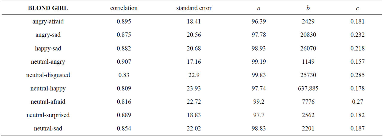
Table 2. Technical characteristics of the 9 logistic curves fitting empirical data: quality of fit (correlation coefficient and standard error) and parameters (a, b, c).
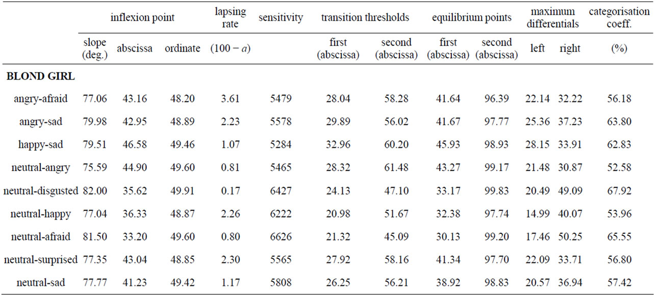
Table 3. Values of the relevant properties of the curves.
inability to make a binary choice. In short, it reflects a conflict or competition between two opposite responses. It seems reasonable to estimate this width by the difference between the abscissas of the two transition thresholds; probably, this difference is dependent of the slope. The mean difference was 27.87 (±2.13) and 28.47 (± 4.11) respectively for unipolar and bipolar ES (about one quarter of the entire 0 - 100 scale), with variations between pairs of expressions. Now, while the neutral/angry series displayed the lowest slope, the slope of the neutral/disgusted series displayed was not the highest one: accordingly, the width of the uncertainty area was not entirely constrained by the slope, even if the slope was probably the major determinant of it (correlation coefficient between the slope and the width of the window = −0.95). We note that the picture formed with 50% of A pixels and 50% of B pixels was situated within the uncertainty window in seven of the nine ES. CP was mainly expected for bipolar series, while this prediction was less valid for unipolar ones. Indeed, in that case what is measured is a kind of absolute threshold on a one-dimensional scale of emotional intensity. Consequently, the slope and the width of the uncertainty window of the unipolar curves should be less important for diagnostic purpose than those of bipolar curves. Also, one can expect that the abscissa of the (virtual) picture leading to 50% of responses B would be lower for unipolar than for bipolar ES. This was not verified, however, as the mean slope of the three bipolar series was 78.84 deg. vs 78.54 for the six unipolar series, the mean width of the window was 27.7 (±2.13) and 28.5 (±4.11) for the bipolar and unipolar series respectively, and the abscissa of the
 (a)
(a)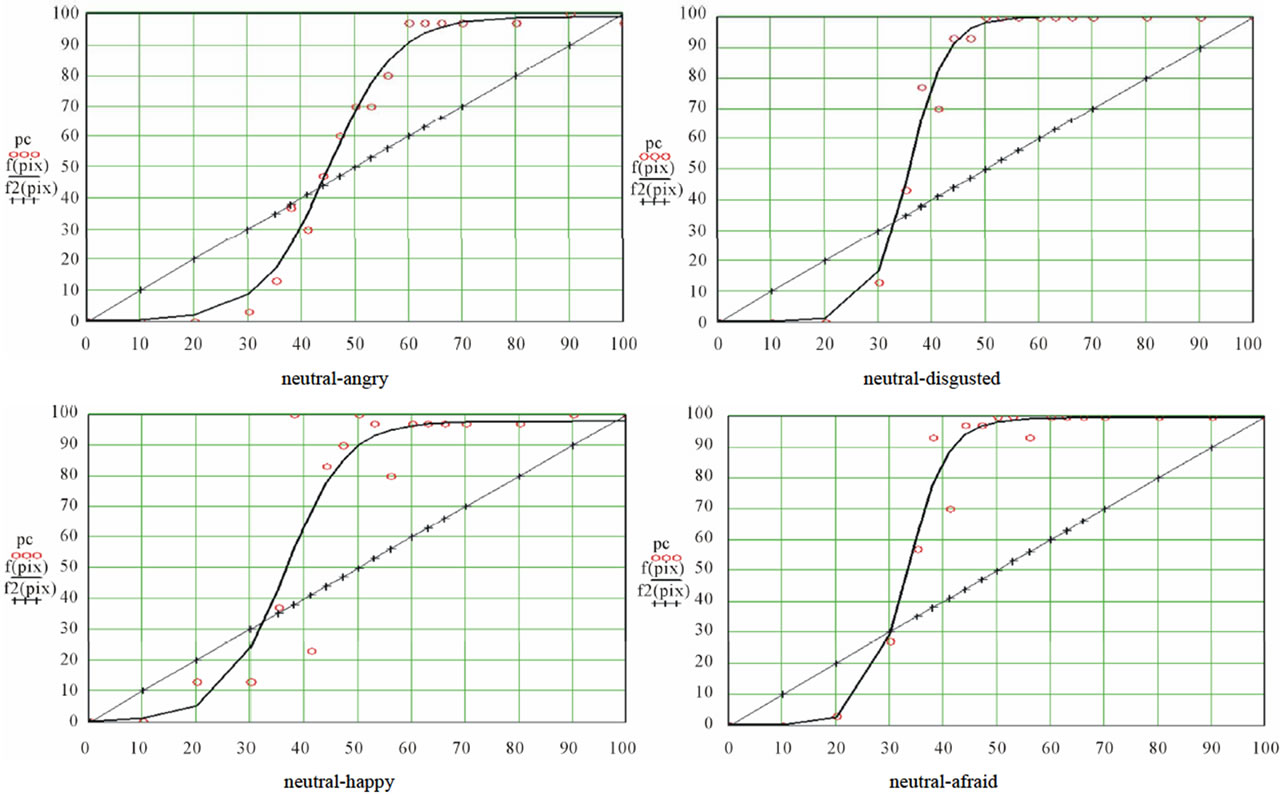 (b)
(b)
Figure 4. (a) Bipolar series. Conversion series of binary responses on MARIE through mathematical model. The measurement of visual recognition of facial emotions among subjects from ages 20 to 30 years; (b) Unipolar series. Conversion series of binary responses on MARIE through mathematical model. The measurement of visual recognition of facial emotions among subjects from ages 20 to 30 years.
uncertainty picture for bipolar ES was 43.08 (±2.46) against 36.53 (±5.36) for unipolar series. Whatever may be the significance of this observation, we note that for series where expression A was of emotional neutrality. CP actually applied, indicating that the classical Fechner’s psychophysical law was not the rule. Indeed, this law establishes that the intensity of the sensation is a logarithmic function of the intensity of the stimulus.
3.6. Conclusions
First, it can be seen that the fit of observed data to data predicted by the logistic function was very good. Secondly, we note that the contribution of pixels B for which half the subjects would chose A and the other half B, was lower than 50, varying between 30.1 and 45.9, which suggests some effects of the ES. Thirdly, the categorical nature of the processing seemed to be well supported, as slopes varied between 75.6 and 82 degrees.
We are convinced that this method of analyzing CP is promising, and overcomes the first challenge mentioned above—namely, to define adequate parameters of the distributions. This mathematical method allows the use of this tool, a potential diagnostic instrument (MARIE), totally independent of 1) the kind of stimuli (visual, auditory, olfactory, and tactile); 2) the number of subjects; and 3) the number of stimuli in the ES. Therefore, one can construct a general graph common to all authors but only dependent on the type of emotions. This will enhance inter-examiner correlation and correspondence yielding uniformity of results independent of variables related to examiners and interactions with examiners. In addition, some parameters are suggested—particularly the maximal slope of the curves, the localization of the point of inflexion, and the lapsing rate that could be used in conventional statistical analysis to compare different conditions with a potential to lead to significant variations of CP. Finally, for the study of the effort involved in double or multiple tasks, a tool like the present one should be of interest for clinical psychiatrists investigating the effects of brain damage and/or aging on the VRFEE or the recognition of facial identities. The application of this tool in geriatric psychiatry could be promising for early detection of dementia of the Alzheimer’s type. This was precisely the purpose of experiment 2.
4. EXPERIMENT 2
4.1. Introduction
In this second step, the results of experiment 1 were used to compare a healthy sample of elderly participants to a matched sample of patients suffering from mild Alzheimer’s Disease (AD). In this pathology, most authors confirm a disorder of VRFEE. As a matter of fact, these groups had been compared in a previous study [32]. However, the statistical approach was used while, in the present study, the mathematical rationale with graphs analysis will be used.
4.2. Participants
So, comparisons of 12 mild AD (DSM IV) to 12 matched controls were made; the matching concerned sex, age and education (see table 4). The 24 subjects were Caucasian, right-handed, and native of northern France. Visual acuity was 20/20. No history of neurological or psychiatric disorder was present, and no psychotropic or neuroleptic medication was used during the six months prior to the experiment. No abnormal behavior was identified since the onset of AD. Patients met the NINCDS-ADRDA criteria for Dementia of the Alzheimer’s type without behavioral disturbance [48]. Signs suggestive of Lewy body disease
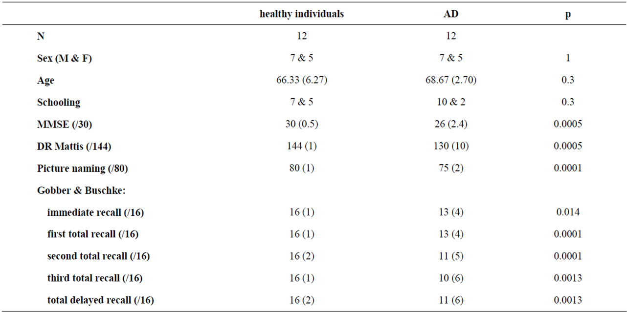
Table 4. Comparison of a healthy sample of elderly participants to a matched sample of patients suffering from mile Alzheimer’s Disease (AD) with the mathematical approach of the battery MARIE. Level of schooling since age 4: 12 years vs 15 years or more; age, MMSE, Mattis, Picture naming, Grober & Buschke: mean (standard deviation).
[49], fronto-temporal cortical atrophy [50,51], or corticobasal degeneration [52] were exclusion criteria. We administered the Mini Mental Status Examination [53], the Mattis Dementia Rating Scale [54,55], the OD80. [56], and the RI/RL-16 battery [57-59] to all participants (see table 4). Our previous statistical analysis [33] had shown an impairment of VRFEE in mild AD with a higher threshold of visual recognition for all emotions, and a difficulty to distinguish anger from fear.
4.3. Results and Discussion
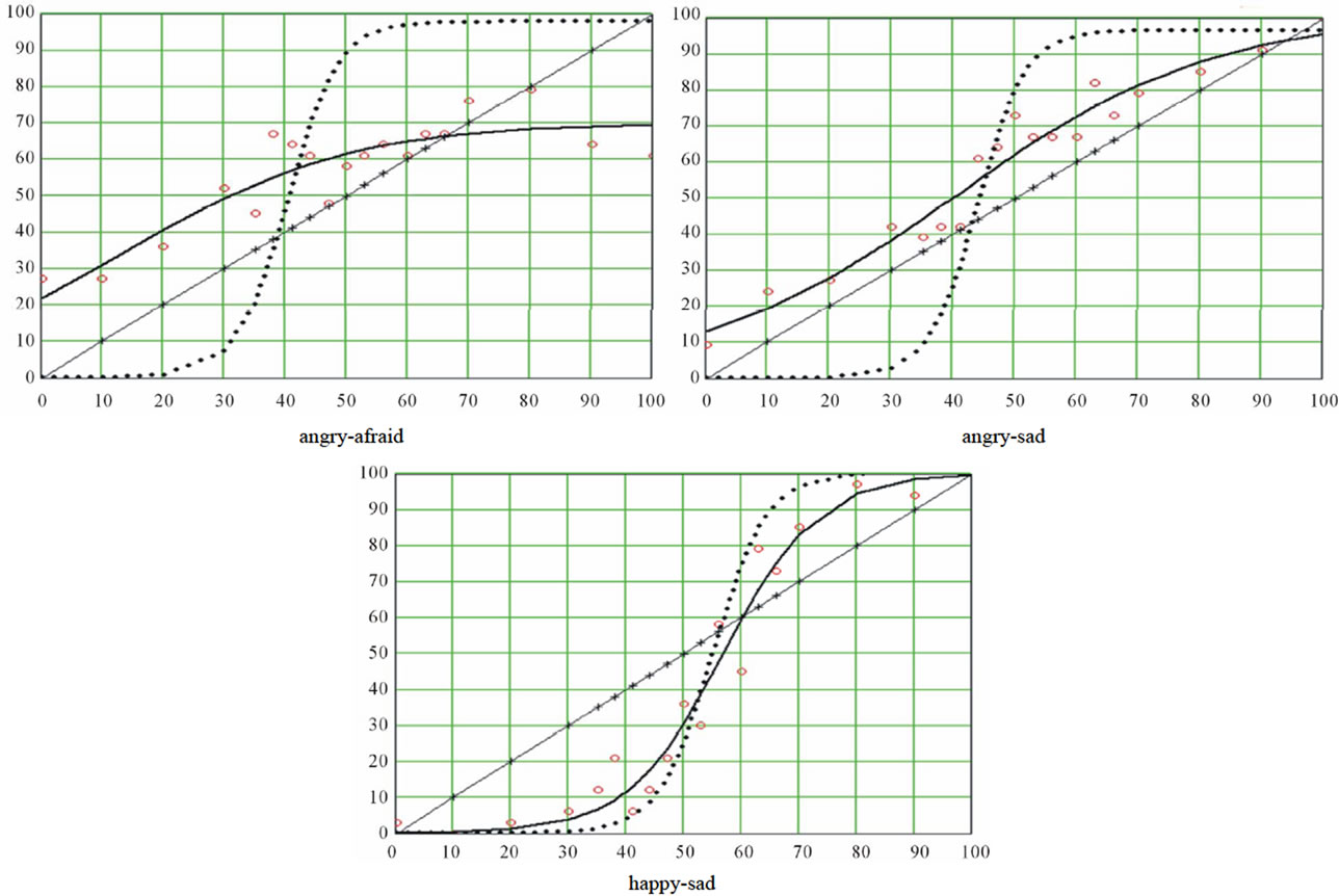
4.3.1. Bipolar Series
Figure 5(a) summarizes all identified parameters and the graphs for the three bipolar series. The angry-afraid series shows no categorization in mild AD. This sample had great difficulty in distinguishing anger from fear. It is not surprising to see the flatness of the curve of mild AD as the responses seem to be given at random. In this case, for each series, one observes 50% responses A and 50% responses B, which provides a flat curve. However, the answers are not completely random because the right half of the curve evidences between 60% and 70% responses B. The confusion between angry and afraid is in favor of afraid. The angry-afraid series appears to be sensitive to early AD.
The series angry-sad shows a diagonal-like curve for mild AD. It is worth observing the proportionality between the percentage of responses B and the percentage of B pixels. This emotional perception is less categorical and rather uni-dimensional in mild AD than in healthy participants. This implies that the categorization seems to be a hallmark of higher cognitive functions. An alteration of cognition leads to a one-dimensional perception of emotions. The happy-sad series is less altered in the mild AD group. In this series, CP appears to be intact and is spared in the mild AD.
4.3.2. Unipolar Series
Figure 5(b) shows the identified parameters and the graphs for the six unipolar series. In mild AD, all curves are shifted to the right. Thus, AD is less sensitive to emotion B than controls. Moreover, all curves tend to become diagonal. Mild AD patients tend to lose their ability to categorize emotions in favor of a one-category perception. The lapsing rate measures the ability to recognize canonical emotions. In the case of a normal recognition, the horizontal portion of the left half is asymptotic to 100% and measures closer to 0. In other words, we have the percentage of subjects who do not recognize the emotion considered as canonical. We find that 6.5%, 2.8%, 5.4%, 2.3% and 2.7% of mild AD do not recognize respectively anger, disgust, happiness, surprise and sadness. Let us note that these patients have scores of 130 ± 10 for DR Mattis, and 26 ± 2.4 for the MMSE. We are at an early stage of AD, and figures 5(a) and (b) show the severity of the deficit of VRFEE. At a more advanced stage of the disease, one can imagine that the patient becomes unable to identify any facial expression. This would confirm the sensitivity of MARIE and the
 (a)
(a)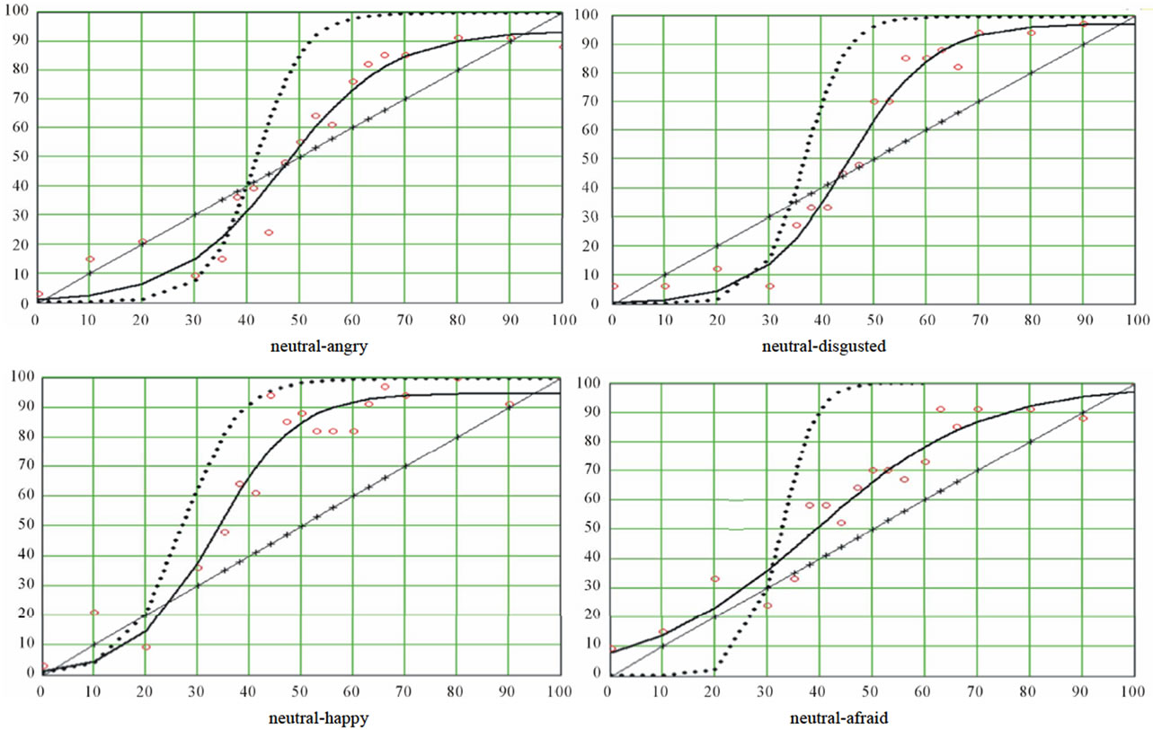 (b)
(b)
Figure 5. (a) Bipolar series. Conversion series of binary responses MARIE through mathematical model. The comparison and measurement of visual recognition of facial emotions among the group of matched healthy subject (dotted) and the group of mild Alzheimer’s Disease (solid line) becomes explicit in terms metrics and graphics terms; (b) Unipolar series. Conversion series of binary responses MARIE through mathematical model. The comparison and measurement of visual recognition of facial emotions among the group of matched healthy subject (dotted) and the group of mild Alzheimer’s Disease (solid line) becomes explicit in terms metrics and graphics terms.
chosen mathematical method associated to it. CP seems to be an attribute of an optimal discrimination of emotions. The disappearance of the categorical perception suggests a functional switch that allows for emotional choice without hesitation. The neuro-fibrillary tangles found in AD settle first in the trans-entorhinal cortex of the hippocampus. This suggests that VRFEE relies on the neural circuitry of procedural Memory in the amygdalohippocampal complex. Disruption of this feature can be attributed to the pathology located in the amygdalohippocampal complex or in the frontal lobe which is the integrative center of emotions.
4.3.3. Conclusions for Clinicians
After experiment 1, the study of mild AD sample matched to a healthy sample (experiment 2) did not pose difficulty. It allowed us to confirm and measure precisely a disorder of VRFEE in mild AD patients. The results are promising because the combination of assessment of VRFEE with a measure of verbal episodic memory could easily suggest the diagnosis of a subclinical AD. Indeed, these two cognitive functions are mediated in large part by the amygdalo-hippocampal complex. Also, the corresponding presence of poor scores on the instruments measuring verbal episodic memory indicate the presence of organic disease of the hippocampus. These scores used together with the assessment of VRFEE could increase and improve the specificity in the diagnostic probability of AD. In addition, these curves allow reflection on the neurobiological underpinnings of AD and recognition of emotions. It is proposed that the loss of VRFEE be called PERCEPTUAL AGNOSOTHYMIA. The difficulties in recognizing facial emotional expressions could explain the self-imposed confinement of patients in their homes, their tendency towards social isolation, and other behavior disorders predicated upon misperceived anger in others when not evident in facial expressions, etc. [56]. All of this can seem unreasonable to casual observers without appreciation of the deficit of this function of CP of emotions in people suffering from AD.
5. GENERAL CONCLUSION
The application of MARIE as a potential diagnostic instrument, and our mathematical method, provide a set of quantitative variables that express one of the cerebral functionalities of the VRFEE. It is intriguing to ponder upon the extreme simplicity of the man-machine interface which is the right and the left mouse button and its use tapping the complexity of the insights gained from resulting outcomes. Remember that the basic principle of computing is a combination and manipulation of 0 and 1. The administration of MARIE is possible even if the patient has low comprehension skills and requires no sophisticated cognitive abilities. In addition to its use in the cognitive dimension, it seems to us that MARIE is a tool which will make it possible to explore more precisely the operations of the brain in its emotional dimension. The ease and speed of this tool has to be taken into consideration. It will allow the scientific, objective study of a cerebral function which is extremely subjective. It can be applied in the medical, psychological, and social field. It will confirm or disprove the work of Ekman [29] on the universal aspect of the visual recognition of facial emotions. This methodology with the use of the proposed mathematical model allowed measuring the performance of an individual who recognizes an emotion by establishing a reference range for the normal population [25].
6. ACKNOWLEDGEMENTS
This work was supported by the grant 1998/1954 of the Programme hospitalier de recherche clinique of the French government. Thanks are due to Paul Ekman who gave permission to use photographs from “Unmasking the faces” (Ekman & Friesen, 1975) and to Olivier Lecherf who designed the computer program for processing and displaying the pictures. This study was made possible thanks to the Centre d’-Investigation Clinique (CIC-CHU/INSERM, Lille). I thank Mr. JAHAN Philippe Director of the Centre Hospitalier de Valenciennes, Dr. CUINGNET Philippe and Dr. SABOUNTCHI Thierry for their aid and support. MARIE is a registered trademark. For an online testing go to www.marie-emotion.
REFERENCES
- Beale, J.M. and Keil, F.C. (1995) Categorical effects in the perception of faces. Cognition, 57, 217-239. doi:10.1016/0010-0277(95)00669-X
- Bornstein, M.H., Kessen, W. and Weiskopf, S. (1976) The categories of hue in infancy. Science, 191, 201-202. doi:10.1126/science.1246610
- Calvo, M.G. and Nummenmaa, L. (2011) Time course of discrimination between emotional facial expressions: The role of visual saliency. Vision Research, 51, 1751-1759. doi:10.1016/j.visres.2011.06.001
- Harnad, S. (1987) Categorical perception: The groundwork of cognition. Cambridge University Press, Cambridge.
- Levin, D.T. and Beale, J.M. (2000) Categorical perception occurs in newly learned faces, other-race faces, and inverted faces. Perception & Psychophysics, 62, 386-401. doi:10.3758/BF03205558
- Pollak, S.D. and Kistler, D.J. (2002) Early experience is associated with the development of categorical representations for facial expressions of emotion. Proceedings of the National Academy of Sciences, 99, 9072-9076. doi:10.1073/pnas.142165999
- Rossion, B. (2002) Is sex categorization from faces really parallel to face recognition? Visual Cognition, 9, 1003-1020. doi:10.1080/13506280143000485
- Rossion, B., Schiltz, C., Robaye, L., Pirenne, D. and Crommelinck, M. (2001) How does the brain discriminate familiar and unfamiliar faces? A PET study of face categorical perception. Journal of Cognitive Neuroscience, 13, 1019-1034. doi:10.1162/089892901753165917
- Treisman, M.A., Faulkner, A., Naish, P.L.N. and Rosner, B.S. (1995) Voice-onset time and tone-onset time: The role of criterion-setting mechanisms in categorical perception quarterly. Journal of Experimental Psychology, 48, 334-366. doi:10.1080/14640749508401394
- Young, A.W., Rowland, D., Calder, A.J., Etcoff, N.L., Seth, A. and Perrett D.I. (1997) Facial expression megamix: Tests of dimensional and category accounts of emotion recognition. Cognition, 63, 271-313. doi:10.1016/S0010-0277(97)00003-6
- De Gelder, B. and Vroomen, J. (2000) The perception of emotions by ear and by eye. Cognition & Emotion, 14, 289-311. doi:10.1080/026999300378824
- De Gelder, B., Vroomen, J., De Jong, S.J., Masthoff, E., Trompenaars, F.J. and Hodiamont, P. (2005) Multisensory integration of emotional faces and voices in schizophrenics. Schizophrenia Research, 72, 195-203. doi:10.1016/j.schres.2004.02.013
- Fry, D.B., Abramson, A.S., Eimas, P.D. and Liberman, A.M. (1962) The identification and discrimination of synthetic vowels. Language and Speech, 5, 171-189.
- Guenter, F.H., Husain, F.T., Cohen, M.A. and ShinCunningham, B.G. (1999) Effects of categorization and discrimination training on auditory perceptual space. Journal of the Acoustical Society of America, 106, 2900-2912. doi:10.1121/1.428112
- Liberman, A.M., Harris, S., Hooman, H.S. and Griffith, B.C. (1957) The discrimination of speech sounds within and across phoneme boundaries. Journal of Experimental Psychology, 54, 358-368. doi:10.1037/h0044417
- Lisker, L. and Abramson A. (1964) A cross-language study of voicing in initial stops. Word, 20, 384-422.
- Neary, T.M. and Hogan, J.T. (1986) Phonological contrast in experimental phonetics: Relating distributions of production data to perceptual categorical curves. In: Ohala, J.J. and Jaeger, J.J., Eds., Experimental Phonology, Academic Press, Orlando, 141-161.
- Boynton, R.M. and Gordon, J. (1965) Bezold-Brücke hue shift measured by color-naming technique. Journal of the Optical Society of America, 55, 78-86. doi:10.1364/JOSA.55.000078
- Bülthoff, I. and Newell, F.N. (2004) Categorical perception of sex occurs in familiar but not unfamiliar faces. Visual Cognition, 11, 823-855. doi:10.1080/13506280444000012
- Calder, A.J., Keane, J., Manly, T., Sprengelmeyer, R., Scott, S., Nimmo-Smith, I. and Young, A.W. (2003) Facial expression recognition across the adult life span. Neuropsychologia, 41, 195-202. doi:10.1016/S0028-3932(02)00149-5
- Etcoff, N.L. and Magee, J.J. (1992) Categorical perception of facial expressions. Cognition, 44, 222-240. doi:10.1016/0010-0277(92)90002-Y
- Shah, R. and Lewis, M.B. (2003) Locating the neutral expression in the facial-emotion space. Visual Cognition, 10, 549-566. doi:10.1080/13506280244000203a
- Stevenage, S.V. (1998) Which twin are you? A demonstration of induced categorical perception of identical twin faces. British Journal of Psychology, 89, 39-57. doi:10.1111/j.2044-8295.1998.tb02672.x
- Bruyer, R. and Granato, P. (1999) Categorical ef-fects in the perception of facial expressions: MARIE A simple and discriminating clinical tool. European Review of Applied Psychology, 49, 3-10.
- Bruyer, R., Granato, P. and Van Gansberghe, J.P. (2007) An individual recognition score of a series of intermediate stimuli between two sources: Categorical perception of facial expressions (in French). European Review of Applied Psychology, 57, 37-49. doi:10.1016/j.erap.2006.02.001
- Campanella, S., Chrysochoos, A. and Bruyer, R. (2001) Categorical perception of facial gender information: Behavioural evidence and the face-space metaphor. Visual Cognition, 8, 237-262. doi:10.1080/13506280042000072
- Dampe, R.I. and Harnad, S.R. (2000) Neural network models of categorical perception. Perception & Psychophysics, 62, 843-867. doi:10.3758/BF03206927
- De Gelder, B., Teunisse, J.P. and Benson, P.J. (1997) Categorical perception of facial expressions: Categories and their internal structure. Cognition & Emotion, 11, 1-23. doi:10.1080/026999397380005
- Ekman, P. and Friesen, W.V. (1975) Unmasking the face. Prentice Hall, Englewood Cliffs.
- Granato, P., Bruyer, R. and Revillion, J.J. (1996) “Étude objective de la perception du sourire et de la tristesse par la méthode d’analyse de recherche de l’intégration des émotions MARIE. Annales Médico-Psychologiques, 154, 1-9.
- Granato, P. and Bruyer, R. (2002) Measurement of facially expressed emotions by a computerized study: Method of study and analysis of integration of emotions (MARIE). European Psychiatry, 17, 339-348. doi:10.1016/S0924-9338(02)00684-3
- Granato, P., Godefroy, O., Van Gansbergh, J.P. and Bruyer, R. (2009) Impaired facial emotion recognition in mild Alzheimer’s disease. La Revue de Gériatrie, 34, 853-859.
- Granato, P. (2007) La perception visuelle des émotions faciales caractéristiques de la population générale et perturbations liées à la schizophrénie et à la maladie d’Alzheimer. Thesis, University Lille, Lille.
- Hsu, S.M. and Young, A.W. (2004) Adaptation effects in facial expression recognition. Visual Cognition, 11, 871-899.
- Huang, J., Chan, R.C.K., Gollan, J.K., Liu, W., Ma, Z., Li, Z. and Gong, Q. (2011) Perceptual bias of patients with Schizophrenia in morphed facial expression. Psychiatry Research, 185, 60-65. doi:10.1016/j.psychres.2010.05.017
- Calder, A.J., Young, A.W., Perrett, D.I., Etcoff, M.L. and Rowland, D. (1996) Categorical perception of morphed facial expressions visual. Cognition, 3, 81-117. doi:10.1080/713756735
- Gourevitch, V. and Galanter, E. (1967) A significance test for one-parameter isosensitivity functions. Psychometrika, 32, 25-33. doi:10.1007/BF02289402
- Hardin, J.W. and Hilbe, J. (2003) Generalized estimating equations. CRC Press, Boca Raton.
- Hosmer, D.W. and Lemeshow, S. (2000) Applied logistic regression. 2nd Edition, Wiley, New York. doi:10.1002/0471722146
- Kaernbach, C. (2001) Slope bias of psycho-metric functions derived from adaptive data. Perception & Psychophysics, 63, 1389-1398. doi:10.3758/BF03194550
- Kee, K.S., Horan, W.P., Wynn, J.K., Mintz, J. and Green, M.F. (2006) An analysis of categorical perception of facial emotion in schizophrenia. Schizophrenia Research, 87, 228-237. doi:10.1016/j.schres.2006.06.001
- Klein, S.A. (2001) Measuring, estimating, and understanding the psychometric function: A commentary. Perception & Psychophysics, 63, 1421-1455. doi:10.3758/BF03194552
- Powers, D.A. and Xie, Y. (2000) Statistical methods for categorical data analysis. Academic Press, San Diego.
- Selvin, S. (2004) Biostatistics. Pearson Education Inc., Boston.
- Strasburger, H. (2001) Converting between measures of slope of the psychometric function. Perception & Psychophysics, 63, 1348-1355. doi:10.3758/BF03194547
- Wichmann, F.A. and Hill, N.J. (2001) The psychometric function: I. Fitting, sampling and goodness of fit. Perception & Psychophysics, 63, 1293-1313. doi:10.3758/BF03194544
- More, J.J. (1978) The Levenberg-Marquardt algorithm: Implementation and theory. In: Watson, G.A., Ed., Numerical Analysis, Springer, Berlin, 105-116.
- Mc Khann, G., Drachman, D., Folstein, M., Katzman, R., Price D. and Stadlan, E.M.(1984) Clinical diagnosis of Alzheimer’s disease: Report of the NINCDS-ADRDA Work Group under the auspices of Department of Health and Human Services Task Force on Alzheimer’s Disease. Neurology, 34, 939-944.
- Mc Keith, I.G. (2004) Advances in the diagnosis and treatment of dementia with Lewy bodies. Introduction. Dementia Geriatric Cognition Disorder, 1, 1-2.
- Mesulam, M.M. (2001) Primary progressive aphasia. Annals of Neurology, 49, 425-432. doi:10.1002/ana.91
- Snowden, J.S. and Neary, D. (1993) Progressive language dysfunction and lobar atrophy. Dementia, 4, 226-231.
- Caselli, R.J., Jack, C.R. Jr., Petersen, R.C., Wahner, H.W. and Yanagihara, T. (1992) Asymmetric cortical degenerative syndromes: Clinical and radiologic correlations. Neurology, 42, 1462-1468. doi:10.1212/WNL.42.8.1462
- Folstein, M.F., Folstein, S.E. and McHugh, P.R. (1975) Mini-Mental State: A practical method for grading the cognitive state of patients for the clinician. Journal of Psychiatric Research, 12, 189-198. doi:10.1016/0022-3956(75)90026-6
- Lucas, J.A., lvnik, R.J., Bohac, D.L., Tangalos, E.G. and Kokmen, E. (1998) Normative data for the Mattis Dementia rating scale. Journal of Clinical and Experimental Neuropsychology, 20, 536-547. doi:10.1076/jcen.20.4.536.1469
- Mattis, S. (1976) Mental status examination for organic mental syndrome in elderly patients. In: Bellak, L. and Karasu, T.E., Eds., Geriatric Psychiatry, Grune & Stratton, New York.
- Deloche, G., Hannequin, D., Dordain, M., Perrier, D., Pichard, B. and Quint, S. (1996) Picture confrontation oral naming: Performance differences between aphasics and normal. Brain Language, 53, 105-120. doi:10.1006/brln.1996.0039
- Grober, E., Buschke, H., Crystal, H., Bang, S. and Dresner, R. (1988) Screening for dementia by memory testing. Neurology, 38, 900-903. doi:10.1212/WNL.38.6.900
- Van Der Linden, M. and GREMEM. (2004) L'évaluation des troubles de la mémoire—Présentation de quatre tests de mémoire épisodique (avec leur étalonnage). Solal Collection Neuropsychologie.
- Phillips, L.H., Scott, C., Henry, J.D., Mowat, D. and Bell, J.S. (2010) Emotion perception in Alzheimer’s disease and mood disorder in old age. Psychology Aging, 25, 38-47. doi:10.1037/a0017369
NOTES
*Corresponding author.
#Data Processing Consultant in Mathematics, Unfortunately, JPVG died in May 2005.