Journal of Quantum Information Science
Vol.09 No.01(2019), Article ID:90994,14 pages
10.4236/jqis.2019.91001
Reinforcement Learning with Deep Quantum Neural Networks
Wei Hu1*, James Hu2
1Department of Computer Science, Houghton College, Houghton, NY, USA
2Department of Computer and Information Science, University of Pennsylvania, Philadelphia, PA, USA

Copyright © 2019 by author(s) and Scientific Research Publishing Inc.
This work is licensed under the Creative Commons Attribution International License (CC BY 4.0).
http://creativecommons.org/licenses/by/4.0/


Received: January 7, 2019; Accepted: March 5, 2019; Published: March 8, 2019
ABSTRACT
The advantage of quantum computers over classical computers fuels the recent trend of developing machine learning algorithms on quantum computers, which can potentially lead to breakthroughs and new learning models in this area. The aim of our study is to explore deep quantum reinforcement learning (RL) on photonic quantum computers, which can process information stored in the quantum states of light. These quantum computers can naturally represent continuous variables, making them an ideal platform to create quantum versions of neural networks. Using quantum photonic circuits, we implement Q learning and actor-critic algorithms with multilayer quantum neural networks and test them in the grid world environment. Our experiments show that 1) these quantum algorithms can solve the RL problem and 2) compared to one layer, using three layer quantum networks improves the learning of both algorithms in terms of rewards collected. In summary, our findings suggest that having more layers in deep quantum RL can enhance the learning outcome.
Keywords:
Continuous-Variable Quantum Computers, Quantum Machine Learning, Quantum Reinforcement Learning, Deep Learning, Q Learning, Actor-Critic, Grid World Environment

1. Introduction
The society of today is rich in data, generated by all sorts of devices at an unprecedented rate. Knowing how to make good use of this big data has become an urgent and interesting topic. Machine learning (ML) is about teaching computers how to learn from data without being explicitly programmed, and as such the first step of ML is obviously the representation of data in terms of features that computers can understand and process. In the old days of ML, hand-crafted feature extraction was the norm. But today, deep learning uses multilayer neural networks to automatically learn the best features that represent the given data. For this purpose, convolutional neural networks (CNN), recurrent neural networks (RNN) and many more were created. Typically, CNNs excel at extracting features of image data, and RNNs for sequential data. Deep learning has demonstrated its power in broad applications, such as speech recognition, computer vision, and natural language processing. A deep neural network is able to process the input data in multiple processing layers. Each layer has a non-linear activation function and the sequence of these layers leads to learning different levels of abstraction of the input data. The nonlinear activation function offers the expressivity of the whole neural network, which has been a challenge for researchers trying to design similar nonlinear functions on a discrete qubit based quantum computer [1] .
In general, ML can be classified into three categories: supervised learning, unsupervised learning, and reinforcement learning (RL) [2] . The functionality of RL is in between supervised and unsupervised learning. In supervised learning, a ground-truth label is given for each training example and in unsupervised learning one has no labels at all. However, in RL, rewards are provided as some sort of sparse and time-delayed labels and furthermore rewards are given from interaction with the environment. We can say that supervised learning is building a relation between the input and output, but RL is using rewards to build the input-output relation in a sequential trial and error process. RL is the closest to what we might associate with our own learning experience in life, where a positive reward reinforces the current behavior, while a negative reward suggests a change.
Inspired by human and animal behavior of learning from experience, RL is a method of solving sequential decision-making problems with an agent by trial and error in a known (with a model) or unknown (without a model) environment. A model of the environment in RL is an abstraction that an agent can use to predict the responses to its actions from the environment. The aim of RL is to discover optimal policies through interaction with the environment. Given a policy, the agent knows the best action to perform in a specific state. RL enjoys its applications in a wide array of areas including: robotics, recommendation systems, advertising, and stock trading. One of the challenges of RL is that some actions do not get an immediate reward. On the other hand, the reward received by the agent does not completely depend on the current action, but also on some actions in the past. Another difficulty is balancing the exploration vs. exploitation, which means the agent needs to exploit the current best actions to maximize rewards, but also explore new actions that it has not tried to find better actions.
Deep neural networks can approximate any linear or non-linear functions. Based on this property, deep RL uses multilayer neural networks to represent the value function, the policy, and the model in RL [3] [4] . With a combination of deep learning and RL, and by observing just the screen pixels, deep RL computer programs have beaten a world champion in the game Go and played many Atari 2600 video games better than humans [5] [6] [7] . Because of high-dimensional state and action spaces, these problems were previously intractable. In order for an agent to select an action, it has to know the representation of its environment, and this is where deep learning can provide a big help to the agent’s understanding of the environment without expert knowledge and interference. Fortunately, quantum computers can speed up the CPU intensive training of deep neural networks with quantum parallelism.
Quantum computers can make use of the counterintuitive properties of quantum states such as superposition, entanglement, and interference to process quantum information in ways that classical computers cannot. It is well-known that quantum computers can find factors of large integers and search an unstructured database much faster than classical computers. Instead of designing algorithms to process big data on classical computers, there is a new approach to deal with issues of big data using quantum computers. For example, the curse of dimensionality is a serious problem in ML for classical computers. However, quantum computers can solve this problem with ease using superposition of qubits.
In recent years, researchers have investigated different ways of applying quantum computing to improve classical machine learning algorithms [8] - [24] . Because of the peculiar properties of quantum states, it is reasonable to hope that quantum computers may recognize and classify patterns that classical computers cannot. All these hopes and potentials will surely stimulate the rising of quantum machine learning. However, there are challenges in applying quantum computing to ML. For example, quantum processes are linear and unitary, which facilitates the advantage that quantum operations can be carried out in parallel with linear superposition to achieve quantum parallelism, but also creates a difficulty since nonlinear operations are an indispensable tool in ML, especially in deep learning [1] .
Deep learning is a powerful technique in ML and especially in RL. To further our understanding of applying quantum computing to the area of deep RL, we implement two popular RL algorithms [25] [26] [27] [28] [29] , Q learning and actor-critic (AC), using deep quantum neural networks. Our two quantum algorithms are tested in the gird world environment, in which the agent learns to walk on the grid in a way that maximizes cumulative rewards. This work extends our two previous results that solve the contextual bandit problem and implement Q learning with a single layer of quantum network [21] [22] .
2. Related Work
Quantum ML has risen as an exciting and engaging research area. Neural networks are the most versatile ML technique and as such, it has been a long-time desire and challenge to create neural networks on quantum computers. With the recent advances in continuous-variable (CV) quantum models [30] , it is possible to create neural networks on quantum photonic circuits. The work in [31] builds layers of quantum gates in the CV model where D is an array of displacement gates, are interferometers, S are squeezing gates, and are non-Gaussian gates to have an effect of nonlinearity. It is shown that these layers of quantum networks can carry out the classical machine learning tasks such as regression and classification. It also explains the quantum advantage existent in certain problems, where the quantum networks only need a linear number of resources because of superposition of the quantum states but the classical networks need exponentially many. The key ingredients in this work are implementing the affine transformations with Gaussian gates and nonlinear activation functions with non-Gaussian gates in quantum photonic circuits. Our current study uses the technique in [31] to design quantum networks that implement the Q learning and AC algorithms.
3. Methods
RL is a subfield of machine learning, in which an agent learns how to act by its interaction with the environment. RL algorithms can be classified into two categories: Model-based and Model-free. Model-free algorithms can be further divided into: policy-based (actor), value-based (critic), and a combination of both, actor-critic. In model-based RL, the environment is treated as a model for learning.
Q learning and actor-critic are both used in the famous AlphaGo program. One of the advantages of AC models is that they converge faster than value-based approach such as Q learning, although the training of AC is more delicate. In AC algorithms, the agent is divided into two components, an actor and a critic, where the critic evaluates the actions taken by the actor and the actor updates the policy gradient in the direction suggested by the critic. AC methods can be viewed as a generalized policy iteration, which alternates between policy evaluation (obtaining a value for an action) and policy improvement (changing actions according to the value).
This study leverages deep quantum neural networks to estimate and output the state-action value function in Q learning and the state value function and policy in the AC methods with the state as the input to the networks.
3.1. Grid World Environment
The grid world environment is commonly used to evaluate the performance of RL algorithms. It delays the reward until the goal state is reached, which makes the learning harder. Our grid world is similar to the Frozen Lake environment from gym (https://gym.openai.com/envs/FrozenLake-v0/) but with a smaller size of 2 × 3 while the standard size is 4 × 4. It is a 2 × 3 grid which contains four possible areas―Start (S), Frozen (F), Hole (H) and Goal (G) (Figure 1). The

Figure 1. The grid world of size 2 × 3 used in this study, which has 6 possible states and 4 possible actions. Each grid (state) is labeled with a letter which has the following meaning: Start (S), Frozen (F), Hole (H) and Goal (G). The state G has a reward of one and other states have a reward of zero.
agent can move up, down, left, or right directions by one grid square. The agent attempts to walk from state S to state G while avoiding the hole H. The reward for reaching the goal is 1, and all other moves have a reward of 0. The visual description of this grid world is in Figure 1.
The standard Frozen Lake environment can be slippery or not. If it is slippery, any move in the intended direction is successful only at a probability of 1/3 and slides to either perpendicular direction with also a probability of 1/3 (there are two such directions). One episode is defined as a trial by the agent to walk from state S to a terminal state of either H or G. The goal of the agent is to learn what action to take in a given state that maximizes the cumulative reward, which is formulated as a policy that maps states to actions.
3.2. Deep Q Learning
A frequently used term in RL is the return, which is defined as follows:
(1)
where is a reward at time t and is a discount rate . The discount used in the return definition implies that current rewards are more significant than those in the future. Another useful concept in RL is the Q function that can be formulated as below:
(2)
where the expectation is taken over potentially random actions, transitions, and rewards under the policy π. The value of Q(s, a) represents the maximum discounted future reward when an agent takes action a in state s.
Q learning [25] [26] is a critic-only method that learns the Q function directly from the experience using the following updating rule, known as Bellman equation [32] :
(3)
where the max is taken over all the possible actions in state [0, 1) is the discount factor, and α (0, 1] is the learning rate. The sum of the first two terms in the square bracket in Equation (3) is called the target Q value and the third term is the predicted Q value.
In simple RL problems, a table is sufficient to represent the Q function, however, in more complicated problems, a neural network is used instead to represent the Q function as Q(s, a; θ ), where θ is a collection of parameters for the network. Deep Q learning employs multilayer neural networks to approximate the Q function.
The training of this network is to reduce the gap between the predicted Q value and the target Q value as a regression problem by optimizing θ. It is clear that updating θ may cause changes to both values. In a difficult RL problem, other heuristic techniques have to be used in order to stabilize the convergence of the network during training such as experience replay, which breaks the correlations between consecutive samples and uses a fixed target network to stabilize the policy [6] .
In RL, the behavior policy is the one that the agent uses to generate the samples, and the target policy is the one that is being learned. When an RL algorithm can use a different behavior policy from its target policy, it is called off-policy, otherwise on-policy. Q learning is off-policy. The AC methods can be made off-policy, which offers the benefit of learning one policy while using a different behavior policy.
3.3. Deep Actor-Critic Methods
RL algorithms usually fall into three categories: actor-only (policy based), critic-only (value based), and actor-critic methods. Actor-only methods usually parameterize the policy, and then optimize it with a policy gradient. This approach can handle continuous states and actions, but the gradient can have high variance. On the other hand, critic-only methods typically estimate the state-action value function, from which we can find an optimal action, but a difficult step when the action space is continuous. When actions are discrete, one strategy to get a policy or to improve the policy is using . However, when actions are continuous, this technique requires a global maximization at every step. The alternative is to use the gradient of Q to update the policy instead of maximization of Q.
In AC, the agent is composed of an actor and a critic, interacting with an environment, which provides a structure to explicitly represent the policy independent of the value function. The aim of the learning is to tune the parameters θ and in the agent in order to receive maximum average reward. The work of the critic reduces the variance of the policy gradient in the actor so the whole algorithm is more stable than a pure policy gradient method. The implementation of AC can be one network with two outputs or two networks, or even the critic can be a lookup table, and training is done in batch or online.
A schematic illustration of the dynamics in the AC algorithms between the actor, the critic, and the environment is shown in Figure 2, where the agent uses the value (the critic) to update the policy (the actor).

Figure 2. The actor-critic reinforcement learning architecture, in which the agent is made of two components: actor and critic. The responsibility of the actor is to act and the critic is to evaluate the action in the form of a scalar value that the critic sends to the actor. After taking an action by the actor, the reward and next state are sent to the critic but only the next state is sent to the actor. An RL makeup has two components, an agent and an environment. The agent acts on the environment while the environment serves as the object to receive the actions.
We explain the actor-critic algorithms [27] [28] [29] in the episodic environment which has a well-defined end point. Recall that a policy is a probability distribution over actions given some input state. We introduce a parameter θ to the policy function and another parameter to the value function which is the expected sum of rewards when starting in state s and following the policy . Running one episode can generate one whole trajectory of the agent which is recorded as . The policy objective function is defined as where is a reward function. Using a common trick of , the actor-critic algorithm can be stated as the following:

The expression in the AC definition above is usually named advantage in policy gradient algorithms, which suggests the needed amount of change to the gradient, based on the baseline value .
3.4. Deep Quantum Neural Networks in Q Learning and Actor-Critic
For a problem with a small number of states and actions, tables could be used to represent the Q function efficiently, but for larger sizes of state and action spaces, they do not scale well. In this case, neural networks can be employed to approximate the Q function with Q(s, a; θ) parameterized by θ (Figure 3). Instead of using tables or classical neural networks, we use deep quantum neural networks to approximate the Q function, the actor, and the critic in this report.
The critic learns a value function, which is then used by the actor to update its gradient direction in order to encourage the beneficial actions, consequently improving its policy. Actor-critic methods usually have better convergence properties than critic-only methods. There are two outputs of AC algorithms: one is the Q values for different actions from the actor and the other is the value of being in a state from the critic (Figure 3).
By default, AC learning is on-policy as the critic evaluates whatever policy is currently being followed by the actor. But it can be changed to an off-policy by sampling actions from a different policy and then incorporating that policy into the formula for updating the actor, which provides the advantage of better exploration and the support of experience replay with data generated from another behavior policy [29] . Off-policy methods can learn about an optimal policy while executing an exploratory policy.
The REINFORCE algorithm used in [21] updates its network at the end of an episode while the actor-critic does it at each step in an online fashion. The drawback of REINFORCE is that when there is a mixture of good and bad actions within the sequence of actions of one episode, it is difficult to assign the correct credit to each action given the final episodic reward.
Our study uses layers of quantum neural networks composed of photonic circuits to implement Q learning and actor-critic. The photonic gates in our networks as shown in Figure 3 are important basic units in quantum computation, which control how the networks evolve. Mathematically these gates are unitary matrices, with complex-valued entries. The numerical simulation of our quantum networks is done with the Strawberryfields software [33] , which supports the training of a quantum neural network circuit to generate any quantum states using machine learning.
4. Results
Our quantum Q learning and actor-critic algorithms are evaluated in the grid world environment explained in Section 3.1. The aim of the agent in this grid world is to learn how to navigate from the start state S to the goal state G with a reward of 1 without falling into the hole with a reward of 0. Our purpose is to investigate the power of using quantum neural networks with many layers in RL, so we test our quantum networks with one layer and with three layers respectively.
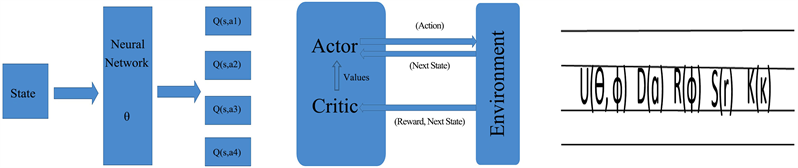
Figure 3. On the left, is the logical representation of the network to compute the Q function (assuming there are 4 actions), in the middle, is the logical representation of the AC model, and on the right, is the physical representation of the actual parametrized circuit structure for a CV quantum neural network made of photonic gates: interferometer, displacement, rotation, squeeze, and Kerr (non-Gaussian) gates. The output is the Fock space measurements. More details of this quantum network can be found in [21] [22] [31] .
Actor-only methods are guaranteed to converge; however, this is not always true for the critic-only methods. The use of a critic causes the AC algorithms to converge faster than the actor-only methods. In certain problems where the action space is much smaller than the state space, the updating of the actor and critic needs more fine-tuning as the learning of a larger space takes more time. The critic computes the advantage, which is a measurement of improvement relative to the baseline value in that state that is also beyond the expected value of that state. To coordinate the work of actor and critic is not easy as seen in Figure 4.
We run several numerical experiments using the Strawberryfields software [33] to simulate our quantum networks, and then take the average of the rewards and path lengths in each case. The results suggest that having more layers in the network can result in better learning. One episode is defined as a sequence of moves from the start state S to a terminal state that can be either the hole H or the goal G in our grid world. The learning curves for the quantum networks of one layer and three layers are displaced respectively in Figure 4. In both Q learning and actor-critic, the networks with three layers converges earlier than the one layer and also more stably. It also seems that in order to avoid the hole H, the agent needs to walk more steps in order to arrive at the goal state G. In other words, earning more rewards requires more work. At the beginning, the agent tends to fall into the hole easily and produces shorter average episode lengths. Only later in the learning, it gradually learns how to avoid the hole.
5. Conclusions
Machine learning teaches computer programs how to improve themselves with experience or data. Therefore, using good features to represent data is essential for ML. Fortunately, deep learning has the ability to automatically extract good features from complex and high-dimensional data, which provides the valuable first step to any real-world applications of RL that require learning from raw visual input.
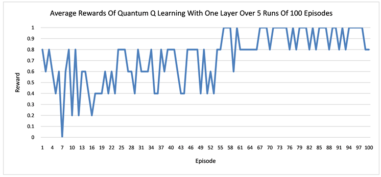
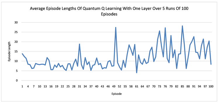
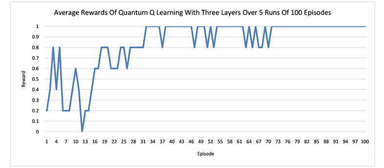
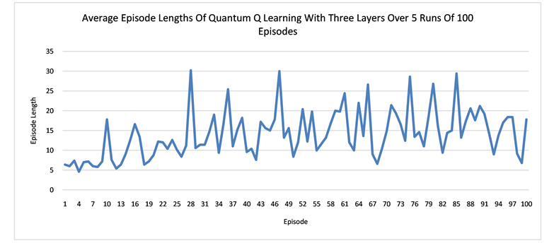
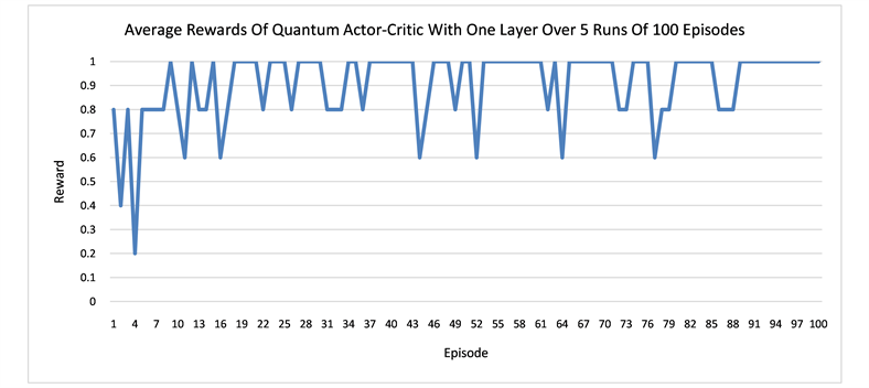
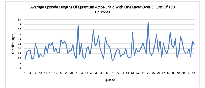
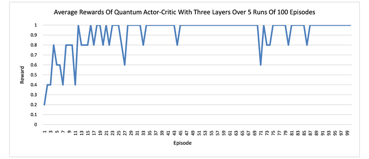
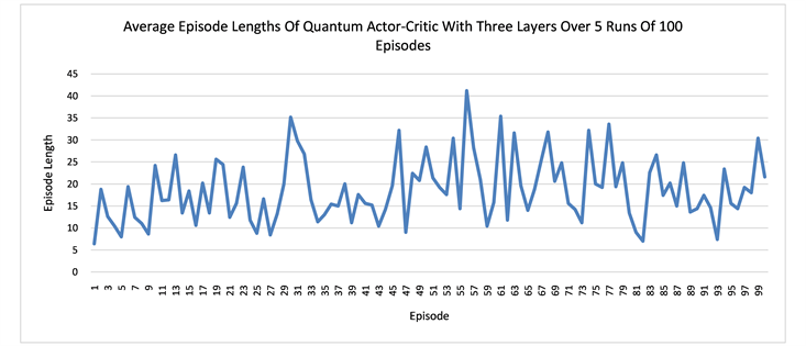
Figure 4. The plots show the learning of the quantum networks in the grid world of size 2 × 3, measured by the average rewards or the episode lengths from state S to state G or H.
Supported by deep learning, RL programs that use Q learning and actor-critic have demonstrated their superior performance, which justifies the call to study these two algorithms on quantum computers. The advantage of having two components, actor and critic, in the AC methods also brings a difficulty in coordinating the work of the two. Relatively speaking, the actor is more sensitive to changes than the critic, as the changes of critic indirectly impact the policy.
Our work shows how to implement Q learning and actor-critic algorithms using deep quantum neural networks. The results of this report highlight that having more layers in the quantum networks does improve the learning of the agent in the grid world environment, which extends our previous work that uses a single layer of quantum network to solve RL problems [21] [22] .
Conflicts of Interest
The authors declare no conflicts of interest regarding the publication of this paper.
Cite this paper
Hu, W. and Hu, J. (2019) Reinforcement Learning with Deep Quantum Neural Networks. Journal of Quantum Information Science, 9, 1-14. https://doi.org/10.4236/jqis.2019.91001
References
- 1. Hu, W. (2018) Towards a Real Quantum Neuron. Natural Science, 10, 99-109. https://doi.org/10.4236/ns.2018.103011
- 2. Sutton, R.S. and Barto, A.G. (2018) Reinforcement Learning. An Introduction. 2nd Edition, A Bradford Book, Cambridge.
- 3. Ganger, M., Duryea, E. and Hu, W. (2016) Double Sarsa and Double Expected Sarsa with Shallow and Deep Learning. Journal of Data Analysis and Information Processing, 4, 159. https://doi.org/10.4236/jdaip.2016.44014
- 4. Duryea, E., Ganger, M. and Hu, W. (2016) Exploring Deep Reinforcement Learning with Multi Q-Learning. Intelligent Control and Automation, 7, 129.
- 5. Mnih, V., Kavukcuoglu, K., Silver, D., Rusu, A.A., Veness, J., Bellemare, M.G., Graves, A., Riedmiller, M., Fidjeland, A.K., Ostrovski, G., Petersen, S., Beattie, C., Sadik, A., Antonoglou, I., King, H., Kumaran, D., Wierstra, D., Legg, S. and Hassabis, D. (2015) Human-Level Control through Deep Reinforcement Learning. Nature, 518, 529-533. https://doi.org/10.1038/nature14236
- 6. Silver, D., Huang, A., Maddison, C.J., Guez, A., Sifre, L., van den Driessche, G., Schrittwieser, J., Antonoglou, I., Panneershelvam, V., Lanctot, M., Dieleman, S., Grewe, D., Nham, J., Kalchbrenner, N., Sutskever, I., Lillicrap, T., Leach, M., Kavukcuoglu, K., Graepel, T. and Hassabis, D. (2016) Mastering the Game of Go with Deep Neural Networks and Tree Search. Nature, 529, 484-489.https://doi.org/10.1038/nature16961
- 7. Silver, D., Schrittwieser, J., Simonyan, K., Antonoglou, I., Huang, A., Guez, A., Hubert, T., Baker, L., Lai, M., Bolton, A., Chen, Y., Lillicrap, T., Hui, F., Sifre, L., van den Driessche, G., Graepel, T. and Hassabis, D. (2017) Mastering the Game of Go without Human Knowledge. Nature, 550, 354-359.https://doi.org/10.1038/nature24270
- 8. Peruzzo, A., McClean, J., Shadbolt, P., Yung, M.-H., Zhou, X.-Q., Love, P.J., Aspuru-Guzik, A. and O’Brien, J.L. (2014) A Variational Eigenvalue Solver on a Photonic Quantum Processor. Nature Communications, 5, Article No. 4213.https://doi.org/10.1038/ncomms5213
- 9. Clausen, J. and Briegel, H.J. (2018) Quantum Machine Learning with Glow for Episodic Tasks and Decision Games. Physical Review A, 97, Article ID: 022303.https://doi.org/10.1103/PhysRevA.97.022303
- 10. Crawford, D., Levit, A., Ghadermarzy, N., Oberoi, J.S. and Ronagh, P. (2016) Reinforcement Learning Using Quantum Boltzmann Machines.
- 11. Dunjko, V., Taylor, J.M. and Briegel, H.J. (2018) Advances in Quantum Reinforcement Learning.
- 12. Biamonte, J., Wittek, P., Pancotti, N., Rebentrost, P., Wiebe, N. and Lloyd, S. (2017) Quantum Machine Learning. Nature, 549, 195-202.https://doi.org/10.1038/nature23474
- 13. Dunjko, V. and Briegel, H.J. (2018) Machine Learning and Artificial Intelligence in the Quantum Domain: A Review of Recent Progress. Reports on Progress in Physics, 81, Article ID: 074001. https://doi.org/10.1088/1361-6633/aab406
- 14. Hu, W. (2018) Empirical Analysis of a Quantum Classifier Implemented on IBM’s 5Q Quantum Computer. Journal of Quantum Information Science, 8, 1-11.https://doi.org/10.4236/jqis.2018.81001
- 15. Hu, W. (2018) Empirical Analysis of Decision Making of an AI Agent on IBM’s 5Q Quantum Computer. Natural Science, 10, 45-58.https://doi.org/10.4236/ns.2018.101004
- 16. Hu, W. (2018) Comparison of Two Quantum Clustering Algorithms. Natural Science, 10, 87-98. https://doi.org/10.4236/ns.2018.103010
- 17. Ganger, M. and Hu, W. (2019) Quantum Multiple Q-Learning. International Journal of Intelligence Science, 9, 1-22. https://doi.org/10.4236/ijis.2019.91001
- 18. Naruse, M., Berthel, M., Drezet, A., Huant, S., Aono, M., Hori, H. and Kim, S.-J. (2015) Single-Photon Decision Maker. Scientific Reports, 5, Article No. 13253. https://doi.org/10.1038/srep13253
- 19. Mitarai, K., Negoro, M., Kitagawa, M. and Fujii, K. (2018) Quantum Circuit Learning.
- 20. Schuld, M. and Killoran, N. (2018) Quantum Machine Learning in Feature Hilbert Spaces. arXiv:1803.07128
- 21. Hu, W. and Hu, J. (2019) Training a Quantum Neural Network to Solve the Contextual Multi-Armed Bandit Problem. Natural Science, 11, 17-27. https://doi.org/10.4236/ns.2019.111003
- 22. Hu, W. and Hu, J. (2019) Q Learning with Quantum Neural Networks. Natural Science, 11, 31-39. https://doi.org/10.4236/ns.2019.111005
- 23. Farhi, E. and Neven, H. (2018) Classification with Quantum Neural Networks on Near Term Processors. arXiv:1802.06002
- 24. Dong, D., Chen, C., Li, H. and Tarn, T.-J. (2008) Quantum Reinforcement Learning. IEEE Transactions on Systems, Man, and Cybernetics, Part B (Cybernetics), 38, 1207-1220.
- 25. Watkins, C.J.C.H. and Dayan (1992) Technical Note: Q-Learning. Machine Learning, 8, 279-292. https://doi.org/10.1007/BF00992698
- 26. Watkins, C.J.C.H. (1989) Learning from Delayed Rewards. PhD Thesis, University of Cambridge, Cambridge.
- 27. Konda, V.R. and Tsitsiklis, J.N. (2003) On Actor-Critic Algorithms. Journal on Control and Optimization, 42, 1143-1166. https://doi.org/10.1137/S0363012901385691
- 28. Grondman, I., Busoniu, L., Lopes, G.A.D. and Babuska, R. (2012) A Survey of Actor-Critic Reinforcement Learning: Standard and Natural Policy Gradients. IEEE Transactions on Systems, Man, and Cybernetics, Part C (Applications and Reviews), 42, 1291-1307.
- 29. Degris, T., White, M. and Sutton, R.S. (2012) Off-Policy Actor-Critic. Proceedings of the 29th International Conference on Machine Learning, Edinburgh, 26 June-1 July 2012, 179-186.
- 30. Serafini, A. (2017) Quantum Continuous Variables: A Primer of Theoretical Methods. CRC Press, London.
- 31. Killoran, N., Bromley, T.R., Arrazola, J.M., Schuld, M., Quesada, N. and Lloyd, S. (2018) Continuous-Variable Quantum Neural Networks.
- 32. Bellman, R. (1957) A Markovian Decision Process. Journal of Mathematics and Mechanics, 6, 679-684.
- 33. Killoran, N., Izaac, J., Quesada, N., Bergholm, V., Amy, M. and Weedbrook, C. (2018) Strawberry Fields: A Software Platform for Photonic Quantum Computing. https://doi.org/10.1512/iumj.1957.6.56038