Open Journal of Statistics
Vol.04 No.09(2014), Article ID:50488,14 pages
10.4236/ojs.2014.49062
Change-Point Analysis of Survival Data with Application in Clinical Trials
Xuan Chen1, Michael Baron2,3
1Department of Biostatistics and Programming, Sanofi, Beijing, China
2Department of Mathematics and Statistics, American University, Washington DC, USA
3Department of Mathematical Sciences, University of Texas at Dallas, Richardson, USA
Email: Xuan.Chen@sanofi.com, baron@american.edu, mbaron@utdallas.edu
Copyright © 2014 by authors and Scientific Research Publishing Inc.
This work is licensed under the Creative Commons Attribution International License (CC BY).
http://creativecommons.org/licenses/by/4.0/


Received 17 July 2014; revised 25 August 2014; accepted 6 September 2014
ABSTRACT
Effects of many medical procedures appear after a time lag, when a significant change occurs in subjects’ failure rate. This paper focuses on the detection and estimation of such changes which is important for the evaluation and comparison of treatments and prediction of their effects. Unlike the classical change-point model, measurements may still be identically distributed, and the change point is a parameter of their common survival function. Some of the classical change-point detection techniques can still be used but the results are different. Contrary to the classical model, the maximum likelihood estimator of a change point appears consistent, even in presence of nuisance parameters. However, a more efficient procedure can be derived from Kaplan-Meier estimation of the survival function followed by the least-squares estimation of the change point. Strong consistency of these estimation schemes is proved. The finite-sample properties are examined by a Monte Carlo study. Proposed methods are applied to a recent clinical trial of the treatment program for strong drug dependence.
Keywords:
Change-Point Problem, Failure Rate, Kaplan-Meier Estimation, Least Squares Estimation, Maximum Likelihood Estimation, Strong Consistency, Survival Function

1. Introduction
Change-point models studied in clinical research usually refer to changes in the failure rate. Many articles and clinical reports describe situations when after a certain survival period, the failure rate is expected to change due to the treatment or during the after-treatment recovery. Detection of such changes, their estimation, and their comparison between different groups of patients (the treatment arm and the placebo arm is the classical example) is important understanding the treatment’s effect and for the evaluation of the treatment’s success. For example, during the zoster pain resolution trial [1] , the treatment lightens pain from acute to subacute and then to chronic, resulting in three different failure rates. As another example, [2] describes analysis of the Physician’s Health Study for testing the effect of beta-carotene on cancer incidence. New tumors need time to become detectable while the treatment does not affect pre-existing tumors. Thus, there is an approximately two-year waiting period before the effect of the treatment is noticeable. Survival times in this example have a higher initial failure rate and a lower failure rate afterwards. Similar examples are found in [3] - [9] .
Survival data with a change point are described by two models for the failure rate, namely, one model before the change point and the other model after the change point. When a subject passes the change point, the failure rate typically reduces, and the probability of the overall survival increases.
This situation is conceptually and mathematically different from the classical change-point model, see e.g. [10] - [14] , where observations follow one distribution before the change point and another distribution after it. In the described scenario, with one or several changes in the failure rate, all the subjects are assumed to have the same distribution. Each change point is understood as a parameter of this distribution that separates two patterns, two different models for the failure rate, and typically, it is the moment of a “clinically significant” reduction of the failure rate.
Despite the fundamental deviation from the classical change-point model, we will show that classical methods for the standard change-point analysis can be to a certain extent applied to the survival data. Developing these methods, we can also account for the right censoring that is typical for survival data.
The goal of this paper is to find efficient change-point detection methods for the piecewise constant failure rate models [5] [6] [8] [15] with unknown pre-change and post-change parameters. Maximum likelihood estimation of the change point in presence of nuisance parameters is reviewed; it appears consistent under certain conditions. A new alternative estimation procedure is proposed based on Kaplan-Meier estimation of the survival function [16] followed by the least-squares estimation of the change point. For this scheme, strong consistency of all the estimators is established. This is a rather constitutive distinction from the classical change-point models where consistent estimation of the change-point parameter is not possible.
Developed methodologies are applied to the recent clinical trial of the treatment program for methamphetamine dependence conducted by Research Across America in Dallas TX [17] . Participants of this trial were characterized by strong addiction to methamphetamine, and the critical measure of efficacy was their time until relapse. Proposed methods show significant change points in the survival function for both control and treatment groups although the change in the treatment group occurs earlier, about two weeks after receiving the treatment. In simple words, it appears that if a regular user of methamphetamine stays away from the drug for two weeks after starting the treatment program, the probability of relapse on any day thereafter reduces significantly. This finding has a rather significant clinical meaning.
The rest of the paper is organized as follows. The failure rate change-point model is introduced in Section 2. In Section 3, we give a brief review of maximum likelihood estimate and its properties. We propose an alternative least square estimator, find its convergence rate, and prove its strong consistency in Section 4. In Section 5, we extend the strong consistency of the least square estimator to a more general model, Cox proportional hazard model with a change point. We compare the two estimation procedures by means of a simulation study in Section 6. Section 7 shows application of these methods to the Prometa clinical trial. Conclusion is given in Section 8. Proofs of theorems, lemmas, and corollaries are in the Appendix section.
2. Survival Models with Change Points
We assume a constant failure rate function  until an unknown time
 . Change occurs at time
 , and
, and  shifts to a new value
  and remains at it thereafter. Thus,
 (1)
(1)
where , and
, and  is the change point, the main parameter of interest.
Consider a sample of  independent subjects with the failure rate function
 . Let
. Let  denote the survival time of subject
 . Survival data are often subject to random right-censoring. If the survival time
  is censored at time
 , the variable

is observed instead of . In practical clinical studies, right-censored survival times are rather common due to the early termination of the observation period or due to patients’ withdrawals from the clinical trial.
The indicator variable

will show whether the  th survival time is censored. Then, we observe pairs
  for
for . Cen- soring variables
  are assumed to be independent of
 . Matthews (1982) and Worsley (1988) discuss the effect of random censorship.
Throughout the paper,  denotes the true value of the change point;
  is the log-likelihood ratio given the occurrence of a change point at
 ;
; ,
,  , and
, and  are the maximum likelihood estimators of
 ,
,  , and
, and , respectively; and
 ,
,  , and
, and  are the proposed least squares estimators of
 ,
,  , and
, and , respec- tively.
3. Maximum Likelihood Estimation
Under model (1), the likelihood function of  is
is

which yields the log-likelihood ratio
 (2)
(2)
where
 (3)
(3)
When  and
and  are known,
  is linear in
 ,
,  is linear between any two consecutively observed survival times, and thus, its maximum is attained at some observed survival time
 , which equals, say, the
  th ordered survival time,
 . For all
 , the value of
  corresponding to the order statistic
  is 0. Hence the maximum likelihood estimator for the change point
  is
is
 (4)
(4)
When  and
and  are unknown, [18] shows that

where  means that the maximum likelihood is attained as
  approaches
  from below, and also proves that
  are consistent.
The effect of random censorship has been studied by many authors. [6] have suggested that moderate censorship has little impact on the null distribution of the likelihood ratio, based on simulation results for type I censoring. [15] have proved that the exact distributions of test statistics under the null hypothesis remain unchanged for type II censoring. For other forms of noninformative censoring [19] have shown that the asymptotic null distributions of likelihood ratio statistics in general remain unchanged.
4. Least Squares Method Based on Kaplan-Meier Estimation
In this section, we introduce a different change-point estimation procedure which is based on Kaplan-Meier estimator of the survival function. Since the Kaplan-Meier method is nonparametric, the change-point estimation scheme proposed here can be easily extended to a wide variety of survival models with change points arising in clinical trials and other applications.
Kaplan and Meier (1958) proposed a famous estimator for the survival function :
:
 (5)
(5)
This is a step function with jumps at observations  for which
 . It is a nonparametric estimator of the survival function, and it can be applied in presence of censoring. No assumptions are required for the probability distribution other than the independence between the survival and censoring variables. Kaplan-Meier estimator (5) has the following properties:
1) It is the nonparametric maximum likelihood estimator of the true survival function .
.
2) It has an asymptotically normal distribution for any  where
where  is continuous.
3) It converges almost surely to  uniformly in
 , and for each
 , there exists
 , such that
 for sufficiently large
 . Refer to [20] for details.
4) If no censoring occurs or all variables are censored at the same time, then the Kaplan-Meier estimator reduces to the usual empirical distribution function.
4.1. Least Squares Estimation and Strong Consistency
Under the piecewise constant failure rate model (1) with a change point , the logarithm of the survival function at the time
  is given as

Let  denote the vector of parameters. Its least squares estimator
  consists of those values of
 ,
,  , and
, and  that minimize the error sum of squares
 (6)
(6)
where
 (7)
(7)
Lemma 1. At , the error sum of squares components satisfy the strong law of large numbers; that is,
  converges to 0 almost surely, as
 .
.
The proof can be found in the Appendix.
To prove the strong consistency of the vector of least squares estimators , we express
  in terms of the residual
 ,
,
 (8)
(8)
where

The uniform convergence of  and the strong law of large numbers in [21] imply directly that
 , (9)
, (9)
 , (10)
 , (11)
 . (12)
Since we assume that there is indeed a change-point, it is reasonable to make the following assumption.
Assumption (A): There exist known  such that
 .
.
Assumption (A) is a classical assumption in the case when a change point is estimated in presence of nuisance parameters, and it ensures that samples of a sufficient size are used to estimate the nuisance parameters.
Under Assumption (A), the least squares estimator  is defined as the minimizer of
  over the given interval, therefore,
 .
.
Theorem 1.  is strongly consistent for
  under Assumption (A).
The proof can be found in the Appendix.
Theorem 2.  is strongly consistent for
  under Assumption (A).
Proof. 1) We will prove  in this part.
We prove by contradiction. Suppose for any , there exist
  and
and  such that
 (13)
(13)
From Theorem 1 and (12), we get
 (14)
(14)
From (13), we have

for all .
.
Also,

Hence, for sufficiently large ,
,

which contradicts (14).
2) We will prove  in this part.
We also prove this by contradiction. Suppose for any , there exist
  and
and  such that
 (15)
(15)
for all .
.
Then

for all .
.
Also,

Hence,

From (11) and Theorem 1, we can get

Hence

whereas

Hence

for sufficiently large , which contradicts Theorem 1.
Combining 1) and 2) gives
 . □
. □
Theorem 3.  is strongly consistent for
  under Assumption (A).
The proof can be found in the Appendix.
4.2. Convergence Rate of the Least Squares Estimator
Now let us investigate the convergence rate of  for known
  and
and . We will analyze the probability that
  is less than
  for
for  outside of the
  -neighborhood of
 , where
  is the true value of the change point.
Theorem 4. For any , there exists
 , such that

for sufficiently large .
.
The proof can be found in the Appendix.
Corollary 1. The change-point estimator  is strongly consistent;
  almost surely as
 . In particular, for any
 , there exists
  such that

for sufficiently large .
.
Proof. According to Theorem 4, for any arbitrary sequence ,
,  as
as , there exists
  such that
 . Hence

Since the sum of probabilities converges, by the Borel-Cantelli lemma, with probability one,  for all
  for sufficiently large
 . Therefore,
  , the minimizer of
 , belongs to the
  -neighborhood of
  almost surely and all sufficiently large
 .
.
It remains to let  go to zero over a countable set (e.g.,
 ). For each
 , we obtain that
  almost surely. Therefore,
  a.s., as
 .
.
5. Least Squares Method for the Cox Proportional Hazard Model with a Change Point
Generalizing the previous results, in this section we develop change-point estimation techniques for a more general model, Cox proportional hazard model with a change point. Under this model, the hazard rate function has the form,
 (16)
(16)
where  is a vector of covariates
 ,
,  are vectors of coefficients, and
  are baseline hazard rates. Clearly, a model with covariates allows to study effects of numerical and categorical factors on the occurrence of a change point and to compare change points between subpopulations.
It is well known that Cox proportional hazard model is semiparametric. Indeed, it puts no assumptions on the form of baseline hazard rates  and
and  (nonparametric part of model) but assumes a parametric form of the effect of covariates on the hazard.
Introduce the following notations:
・  is the hazard function before the change point;
・  is the hazard function after the change point;
・  is the joint likelihood function under model (16);
・  is log-likelihood ratio under model (16);
・  is survival function under model (16);
・  is the unknown parameter vector;
・  is the least squares estimator of
  which, similarly to Section 4.1, minimizes the error sum of squares based on the differences between the log-survival functions obtained from model (16) and from the Kaplan- Meier estimator (5).
Under model (16), the survival function is expressed as

so that

The least squares estimator  of the change point
  and slopes
  and
and  is then defined as the minimizer

of the error sum of squares
 (17)
(17)
where components  are defined in (7).
Strong Consistency and Convergence Rate of the Least Squares Estimator
Extention of the results of Section 4 on the strong consistency of the change point estimator and estimators of the nuisance parameters to Cox proportional hazard model is straightforward. Indeed, the uniform strong consistency of the Kaplan-Meier estimator holds for any type of the underlying distribution of survival times. Therefore, the error sum of squares can be split into four parts as in (8), with almost sure convergence holding for each part.
Along the same lines as in the constant hazard rate model, we obtain the following results.
Lemma 2. At , components of the error sum of squares (17) satisfy the strong law of large numbers; that is,
  converges almost surely to 0 as
 .
.
Theorem 5. With known  and
and , the change-point estimator
  is strongly consistent. It converges to the true change point
  at the same rate as in the constant hazard rate model; i.e., for any
 ,
,

for some  and all sufficiently large n.
Proof. The proof is similar to the proof of Theorem 4.5 and Corollary 4.6 of Section 4.2. □
The following results show that the strong consistency of  holds even without the assumption of known slopes
  and
and .
.
Theorem 6. The estimated slopes  and
and  are strongly consistent for
  and
and  under Assumption (A).
Theorem 7. Under unknown slope parameters  and
and , the change-point estimator
  is strongly consistent under Assumption (A).
Strong consistency of  and
and  in presence of nuisance parameters is proved by the techniques developed in Section 4.1 and essentially along the same lines. For details, see [22] , chapter 5.
6. Comparison of Estimators
In classical cases, under the usual regularity assumptions, the maximum likelihood estimator is asymptotically the uniformly minimum variance unbiased estimator. Change-point models violate the regularity conditions because of the discontinuity of the likelihood function at the change-point parameter. As a result, the maximum likelihood estimator may no longer be optimal. In this section, we compare the maximum likelihood estimator and the least squares estimator by means of the following Monte Carlo simulation study.
Generating samples from model (1) is quite simple. We generate an  sample, and for those vari- ables that exceed
 , replace the generated variable with
 . The memoryless property of Exponen- tial distribution ensures that the resulting variable has the distribution according to (1).
Samples are generated with the change point , censoring time
 , and failure rates
  taken to be
 , and
, and . Clearly, it should be easier to detect the change point if the difference between
  and
and  is larger. Samples sizes from 100 to 300 are considered each with 1000 Monte Carlo runs. An example of ESS, a piecewise polynomial function, is depicted in Figure 1.
Table 1 lists the estimates of ,
,  , and
, and  for different sample size and different actual failure rates. Table 2 lists the mean square errors for estimates of
 ,
,  , and
, and . These estimates and mean square errors lead to the following conclusions:
1) Both MLE and LSE of ,
,  , and
, and  converge to the true change point and hazard rates as the sample size increases.
2) Both MLE and LSE become more accurate when the difference between  and
and  is increased, holding the sample size constant.
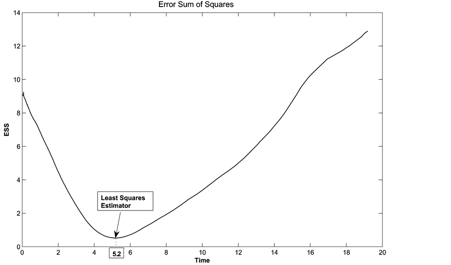
Figure 1. Error sum of squares and the least squares estimator of the change-point.

Table 1. Estimates of ,
,  , and
, and  from simulated data.
Table 2. Mean squared errors of estimates of ,
,  , and
, and .
.
3) The LSE of  has a lower bias than the MLE for the same sample size and the same failure rates. The mean squared error of the LSE of
  is larger than that of the MLE, for the same sample size and same failure rates, however, the hazard rates are estimated by the LSE method with the same or lower mean square error.
7. Example: Prometa Clinical Trial
In this section, we apply both the maximum likelihood method and the least squares method to a recent clinical trial for treating methamphetamine-dependent patients conducted by Research Across America, an outpatient clinical research center in Dallas, Texas [17] .
Fifty patients participated in an open-label study over the time frame of 84 days. In this study, all of the participants were long-term users of methamphetamine. After the screening visit on day 0, patients received five infusions during the first three weeks and conducted 14 follow-up visits.
Later, a double-blind, placebo-controlled study was conducted to better evaluate the effect of treatment. In the double-blind study, neither the participants nor the clinicians knew which patients belong to which treatment arm. The reason for blinding and placebo controls is to determine (as much as possible) whether the effects observed in the study are due to the treatment itself and not other factors. For each participant, the survival time is the time to relapse, which is the duration of time without the use of drugs.
Our goal here is to detect the after-treatment effect of Prometa, which results in a significant reduction of failure rate some time after the first three infusions. We detect such changes with both the maximum likelihood method and the least squares method. Results are listed in Table 3 and Table 4.
First, we estimate the change point for the 50-subject open-label study.
1) Using the maximum likelihood method, day 13 maximizes the log-likelihood ratio in Figure 2, left. The likelihood ratio test provides a p-value of , which is low enough to reject the null hypothesis “there is no change point”. On the day of the change, the failure rate drops from 0.1402 to 0.0105. Thus, we conclude that the failure rate after taking the drugs reduces significantly from 0.1402 to 0.0105 if the patients do not use drugs for 13 days following the treatment.
2) Using the least squares method, the estimate for change point is 14.2373 and the failure rate drops from 0.1281 to 0.0142, which are very close to the results from maximum likelihood estimate. The graph of error sum of squares is in Figure 2, right.
Change points for the female and male groups are compared to see whether occurrence of a change point depends on gender.
1) Using the method of maximum likelihood, the estimated change points for males and females are 8 and 17 from Figure 3, left. However, the likelihood ratio test fails to detect a significant difference between the genders with the p-value of 0.3203, i.e., there is no evidence that there are any significantly different change points for males and females. The failure rate reduces from 0.1649 to 0.0201 for males and from 0.1387 to practically 0 for females.
2) Using the least squares method, the change-point estimator for males is about day 14 and the failure rate reduces from 0.1494 to almost 0, while the change-point estimator for females is 13 and the failure rate reduces from 0.1495 to almost 0. We can see that there is almost no difference between male group and female group in change-point estimators from graph 3, right.
Table 3. Estimates of  for open-label study.
Table 4. Estimates of  for two-armed double-blind study.
Finally, we estimated the change points for the randomized double-blind placebo-controlled study. Change points are estimated separately for the active treatment group and for the placebo group.
1) The graph of log-likelihood ratios is in Figure 4, left. The estimated change point for the treatment group is 13, and the failure rate reduces from 0.0781 to 0.0139. For the placebo group, the change-point estimate is 18, and the failure rate reduces from 0.1145 to 0.0532. The likelihood ratio test shows that these two groups have significantly different change points with p-value 0.0098.
2) With the least squares method, the change-point estimator for the treatment group is around day 17 and the failure rate reduces from 0.0720 to almost 0, while the change-point estimator for Placebo is around 14 and the failure rate reduces from 0.1255 to 0.0016. The graph for error sum of squares is in 4, right.
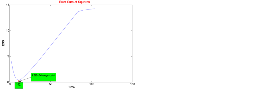
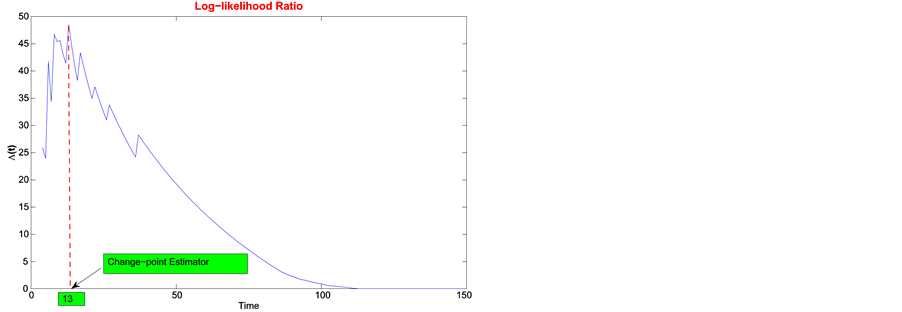
Figure 2. Least squares estimate of change-point for open-label study.
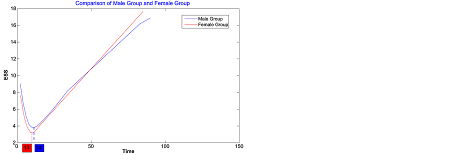
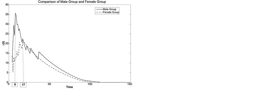
Figure 3. Least squares estimate of change-point for female and male groups.
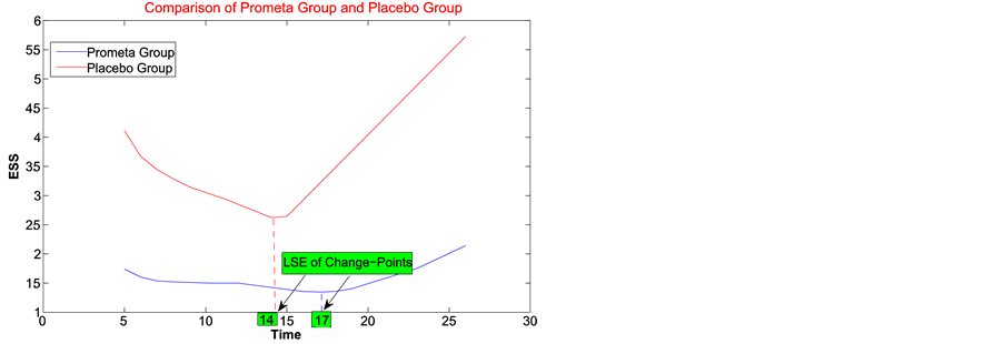
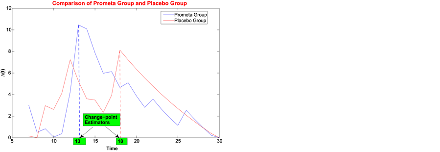
Figure 4. Least squares estimate of change-point for Prometa and Placebo groups.
As a result, besides statistical significance, existence of change-points in the survival curves for both treatment groups has an important clinical significance. It shows a drop in the risk of relapse after a certain period of abstinence. Although the MLE and LSE methods slightly disagree on the exact location of change-points in the two treatment groups, both methods show that the after-change failure rate is significantly lower for the active treatment groups. Essentially, a patient has to abstain from methamphetamine for two weeks after receiving the treatment, and then the failure rate reduces significantly.
8. Conclusion
Detection of change-points in survival curves and estimation of their location finds important application in clinical research. This problem is conceptually different from the standard change-point analysis, where the distribution of data changes at unknown times. Nevertheless, similar statistical techniques can be used. The maximum likelihood approach yields a tractable change-point estimator, however, a more efficient procedure can be obtained by the Kaplan-Meier estimator of the survival function coupled with the method of least squares. Unlike the standard change-point problems, here both methods result in strongly consistent estimators.
Acknowledgements
We thank the Editor and the referee for their comments. Research of M. Baron is funded by the National Science Foundation grant DMS 1322353. This support is greatly appreciated.
References
- Desmond, R.A., Weiss, H.L., Arani, R.B., Soong, S.-J., Wood, M.J., Fiddian, P., Gnann, J. and Whitley, R.J. (2002) Clinical Applications for Change-Point Analysis of Herpes Zoster Pain. Journal of Pain and Symptom Management, 23, 510-516. http://dx.doi.org/10.1016/S0885-3924(02)00393-7
- Zucker, D.M. and Lakatos, E. (1990) Weighted Log Rank Type Statistics for Comparing Survival Curves When There Is a Time Lag in the Effectiveness of Treatment. Biometrika, 77, 853-864. http://dx.doi.org/10.1093/biomet/77.4.853
- Goodman, M.S., Li, Y. and Tiwari, R.C. (2011) Detecting Multiple Change Points in Piecewise Constant Hazard Functions. Journal of Applied Statistics, 38, 2523-2532. http://dx.doi.org/10.1080/02664763.2011.559209
- He, P., Kong, G. and Su, Z. (2013) Estimating the Survival Functions for Right-Censored and Interval-Censored Data with Piecewise Constant Hazard Functions. Contemporary Clinical Trials, 36, 122-127. http://dx.doi.org/10.1016/j.cct.2013.04.009
- Loader, C.R. (1991) Inference for a Hazard Rate Change Point. Biometrika, 78, 749-757. http://dx.doi.org/10.1093/biomet/78.4.749
- Matthews, D.E. and Farewell, V.T. (1982) On Testing for a Constant Hazard against a Change-Point Alternative. Biometrics, 38, 463-468. http://dx.doi.org/10.2307/2530460
- Muller, H.G. and Wang, J.L. (1990) Nonparametric Analysis of Changes in Hazard Rates for Censored Survival Data: An Alternative to Change-Point Models. Biometrika, 77, 305-314. http://dx.doi.org/10.1093/biomet/77.2.305
- Nguyen, H.T., Rogers, G.S. and Walker, E.A. (1984) Estimation in Change-Point Hazard Rate Models. Biometrika, 71, 299-304. http://dx.doi.org/10.1093/biomet/71.2.299
- Sertkaya, D. and Sözer, M.T. (2003) A Bayesian Approach to the Constant Hazard Model with a Change Point and an Application to Breast Cancer Data. Hacettepe Journal of Mathematics and Statistics, 32, 33-41.
- Ahsanullah, M., Rukhin, A.L. and Sinha, B. (1995) Applied Change Point Problems in Statistics. Nova Science Publishers, New York.
- Basseville, M. and Nikiforov, I.V. (1993) Detection of Abrupt Changes: Theory and Application. PTR Prentice-Hall, Inc., Englewood Cliffs.
- Bhattacharya, P.K. (1995) Some Aspects of Change-Point Analysis. In: Change-Point Problems, IMS Lecture Notes- Monograph Series (Vol. 23), 28-56.
- Chen, J. and Gupta, A.K. (2012) Parametric Statistical Change Point Analysis: With Applications to Genetics, Medicine, and Finance. Birkhäuser, Boston. http://dx.doi.org/10.1007/978-0-8176-4801-5
- Poor, H.V. and Hadjiliadis, O. (2009) Quickest Detection. Cambridge University Press, Cambridge.
- Worsley, K.J. (1988) Exact Percentage Points of the Likelihood-Ratio Test for a Change-Point Hazard-Rate Model. Biometrics, 44, 259-263. http://dx.doi.org/10.2307/2531914
- Kaplan, E.L. and Meier, P. (1958) Nonparametric Estimation from Incomplete Observations. Journal of the American Statistical Association, 53, 457-481. http://dx.doi.org/10.1080/01621459.1958.10501452
- Urschel, H.C., Hanselka, L.L., Gromov, I., White, L. and Baron, M. (2007) Open-Label Study of a Proprietary Treatment Program Targeting Type a γ-Aminobutyric Acid Receptor Dysregulation in Methamphetamine Dependence. Mayo Clinic Proceedings, 82, 1170-1178. http://dx.doi.org/10.4065/82.10.1170
- Yao, Y.-C. (1987) Approximating the Distribution of the Maximum Likelihood Estimate of the Change-Point in a Sequence of Independent Random Variables. Annals of Statistics, 15, 1321-1328. http://dx.doi.org/10.1214/aos/1176350509
- Barndorff-Nielsen, O.E. and Cox, D.R. (1984) Bartlett Adjustments to the Likelihood Ratio Statistic and the Distribution of the Maximum Likelihood Estimator. Journal of the Royal Statistical Society: Series B, 46, 483-495.
- Dinwoodie, I.H. (1993) Large Deviations for Censored Data. Annals of Statistics, 21, 1608-1620. http://dx.doi.org/10.1214/aos/1176349274
- Billingsley, P. (1995) Probability and Measure. 3rd Edition, Wiley, New York.
- Chen, X. (2009) Change-Point Analysis of Survival Data with Application in Clinical Trials. Ph.D. Dissertation, The University of Texas at Dallas, Richardson.
Appendix
Proof of Lemma 1
Proof. Express  in the following form,

Define . According to the mentioned uniform convergence of the Kaplan-Meier estimator of the survival function,

and for any , there exists
  such that
 . Hence

Since  minimizes
 , we always have

Hence

Proof of Theorem 1
Proof. From (9), we have

On the other hand,

Hence we have .
.
Proof of Theorem 3
Proof. From Theorems 1, 2, and (10), we obtain

On the other hand,

Hence .
.
Proof of Theorem 4
Proof. First, express  and
and  in terms of the residual
 . From (8),

and

Hence

Let  be the number of
 , and
, and  be the number of
 . For any
  we have the following inequality,

and the theorem is proved.