Open Journal of Statistics
Vol.3 No.6A(2013), Article ID:41359,8 pages DOI:10.4236/ojs.2013.36A001
Subjectivity in Application of the Principle of Maximum Entropy
Measurement Technology, SP Technical Research Institute, Borås, Sweden
Email: peter.hessling@sp.se
Copyright © 2013 Jan Peter Hessling. This is an open access article distributed under the Creative Commons Attribution License, which permits unrestricted use, distribution, and reproduction in any medium, provided the original work is properly cited. In accordance of the Creative Commons Attribution License all Copyrights © 2013 are reserved for SCIRP and the owner of the intellectual property Jan Peter Hessling. All Copyright © 2013 are guarded by law and by SCIRP as a guardian.
Received September 24, 2013; revised October 24, 2013; accepted November 1, 2013
Keywords: Maximum; Entropy; Bayes; Monte Carlo; Uncertainty; Covariance; Deterministic; Sampling; Testable; Information; Model; Calculation; Simulation
ABSTRACT
Complete prior statistical information is currently required in the majority of statistical evaluations of complex models. The principle of maximum entropy is often utilized in this context to fill in the missing pieces of available information and is normally claimed to be fair and objective. A rarely discussed aspect is that it relies upon testable information, which is never known but estimated, i.e. results from processing of raw data. The subjective choice of this processing strongly affects the result. Less conventional posterior completion of information is equally accurate but is computationally superior to prior, as much less information enters the analysis. Our recently proposed methods of lean deterministic sampling are examples of very few approaches that actively promote the use of minimal incomplete prior information. The inherited subjective character of maximum entropy distributions and the often critical implications of prior and posterior completion of information are here discussed and illustrated, from a novel perspective of consistency, rationality, computational efficiency and realism.
1. Introduction
The principle of maximum entropy (PME) can be utilized to determine a probability density distribution function (pdf) from incomplete statistical information. The approach is not limited to determination of prior pdfs in Bayesian estimation, even though that is a common application. It is rather a general recipe how to make known but incomplete statistical information complete with the most ‘fair’ or the weakest possible hypotheses. As such it fits very well into our practice of statistics, where the lack of complete information is the rule rather than the exception. For instance, knowing only the mean and the variance of an uncertain parameter PME results in a normal distribution [1]. The known information must be well defined in a statistical sense, i.e. be formulated in terms of statistical expectations  of functions
  of the considered random quantity
 . For instance,
  yields the mean and
  produces the
  moment around the mean. Their expectations can be estimated from any set of observations
 with estimators [2]
  to give testable information
  [3].
[3].
Bayesian estimation generalizes traditional approaches limited to observations by inclusion of prior knowledge. Its claimed advantage or superiority relies heavily upon fair and truthful assignment of the prior pdf. If the applied method (like PME) to determine the prior pdf turns out to be subjective it would degrade the legitimacy of the approach. Indeed, PME is often motivated by its fairness or objectivity [1]. A minimum of supplementary (unknown) statistical information is imposed by, loosely speaking, maximizing the residual randomness as measured with the information entropy introduced by Shannon [4] and further explored by Jaynes [3]. In practice, the procedure does not provide a complete recipe. By starting with known testable information, PME avoids to define its the best form. There is a widely spread practice though, which probably originates from the ubiquitous use of Taylor expansions. Testable information is usually considered in a hierarchy starting from the mean, the covariance, the skewness, and the kurtosis etc. Various statistical moments around the mean are tested, as if they were terms of a Taylor series. The functions 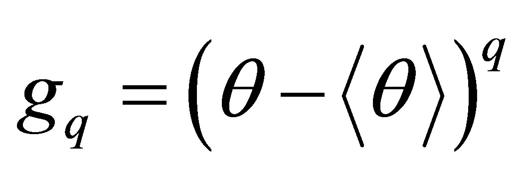 are indeed the
  order monomial related to a Taylor expansion around the mean. The expectation
  will contribute to the nonlinear displacement
 , or scent [5] of
  order, of the model
 . For any other statistic like e.g. covariance, no such simple direct relation holds [6]. Another line of reasoning might be that the mean describes the location of the distribution, the second moment the width, the third the lowest order asymmetry, while the fourth is the lowest order shape indicator etc. We might subjectively claim that these properties (locationwidth-asymmetry-shape) provide a hierarchy of testable information. This does not imply that the moments themselves drop in magnitude or relevance, with their order. On the contrary, the linearly scaled even moments
 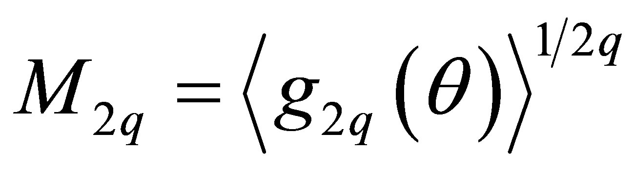 usually increase with the order
 . In the limit
 ,
,  , where
  are the observations of
 .
.
Given a set of observations it is not evident how they should be processed to provide testable information of the highest possible quality, i.e. with minimal residual uncertainty. For instance, which moments  should be estimated with a quality (variance of estimator) that usually decrease with the order
 ? As will be shown, the selection will directly influence the PME distribution function. It is also not evident why PME should be restricted to prior application, as usually practiced. Posterior utilization might in fact simplify the analysis greatly. After all, PME is a general method with no explicit reference to what the distribution describes, the input or the output of the analysis.
2. Method of Maximum Entropy
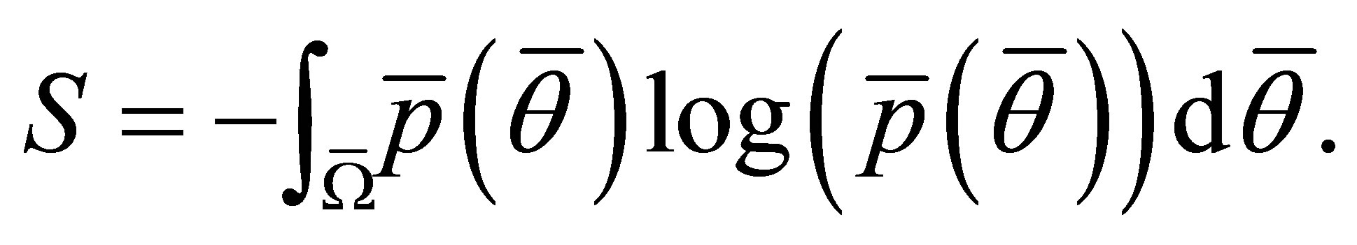
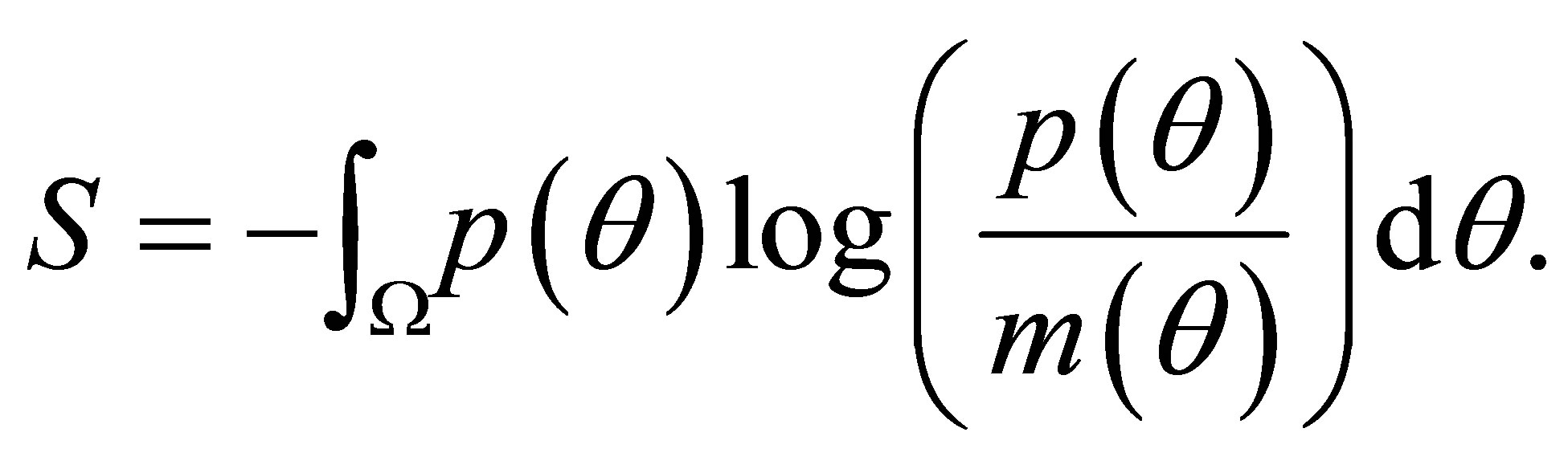
For a continuous sample space , the entropy [4] functional to be maximized in the method of maximum entropy is given by the Lebesgue integral,
 (1.1)
(1.1)
The bar-symbol restricts the integration over distinguishable outcomes . That accounts for our possible ignorance1 of not distinguishing distinct outcomes. As there is an obvious contradiction of being aware of ignorance, it is better translated into irrelevance (for our stated problem). The integration over
  can be extended to
 , by locally measuring the relative density of
  with the Lebesgue measure
 ,
, 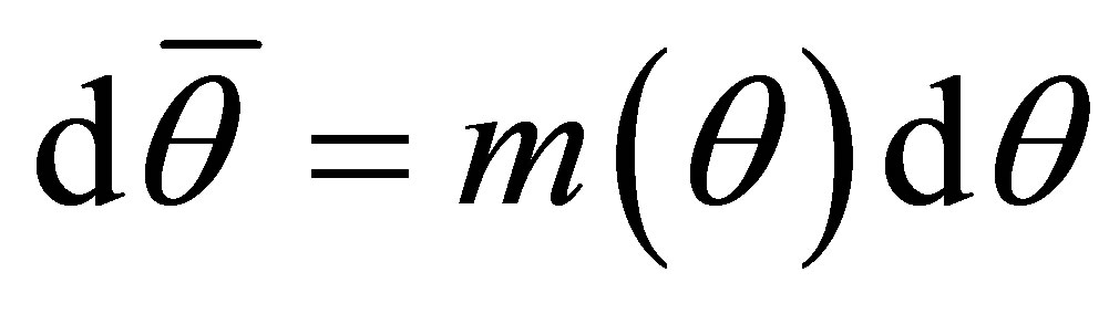 . Consistency requires transformation invariance [1] of the probability
  in the interval
 . That is,
 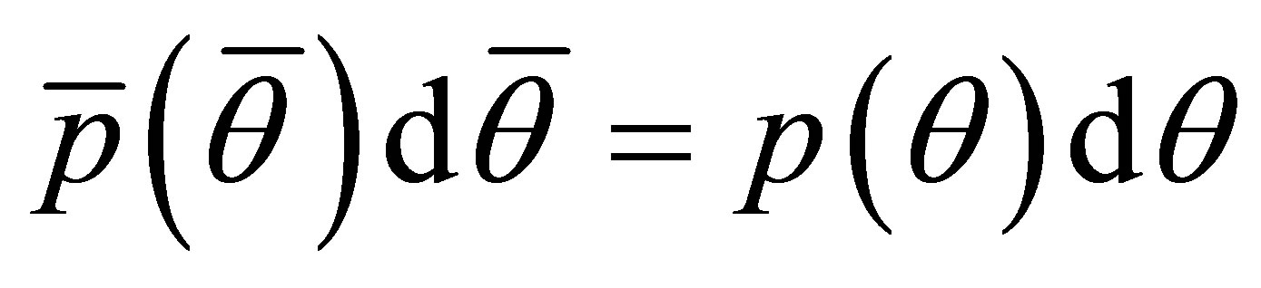 , giving the substitution
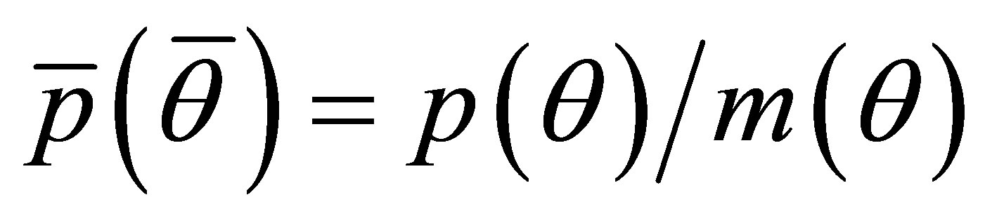 . This invariance is equivalent of requiring independence [3] of
  on the subjectively chosen parameterization. In fact, that constraint provides a direct method of determining the Lebesgue measure: If
 ,
, . For instance, ignorance to change of units correspond to the transformation
 , where
  describes the conversion factor between different units. It yields
  or
or .
.
Utilizing  the integral in Equation (1.1) is converted into a Riemann integral,
 (1.2)
(1.2)
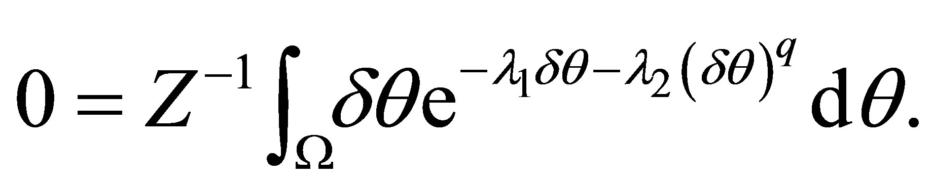
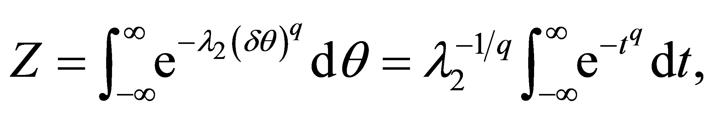
The optimization is subject to all known testable information ,
,
 (1.3)
(1.3)
 (1.4)
(1.4)
The functions  will for convenience be denoted test functions. The mandatory zeroth constraint
  (Equation (1.4)) is the normalization condition. As pointed out [3], for discrete sample spaces and no degeneracy (
 ), there is a general expression for the maximum of Equation (1.1) in terms of a partition function
 . It can be generalized to non-constant measures
 , and continuous distributions using calculus of variations [7],
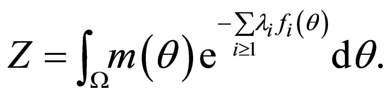 (1.5)
(1.5)
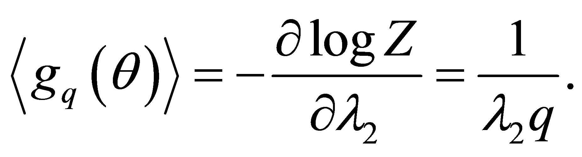
The Lagrange multipliers of optimization are implicitly given by the testable information,
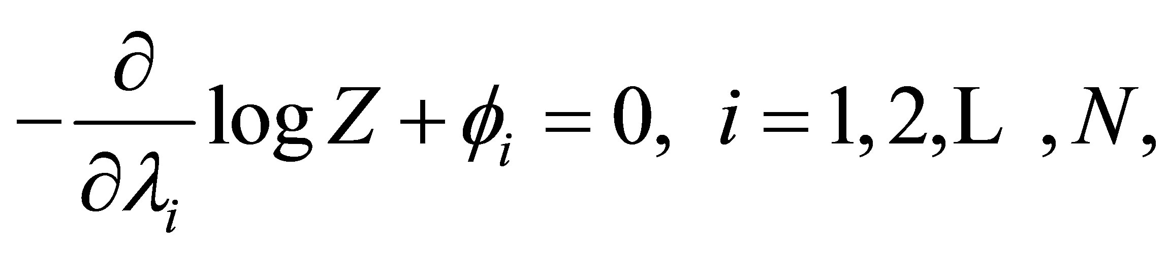 (1.6)
(1.6)
 (1.7)
(1.7)
The maximum entropy pdf is then given by,
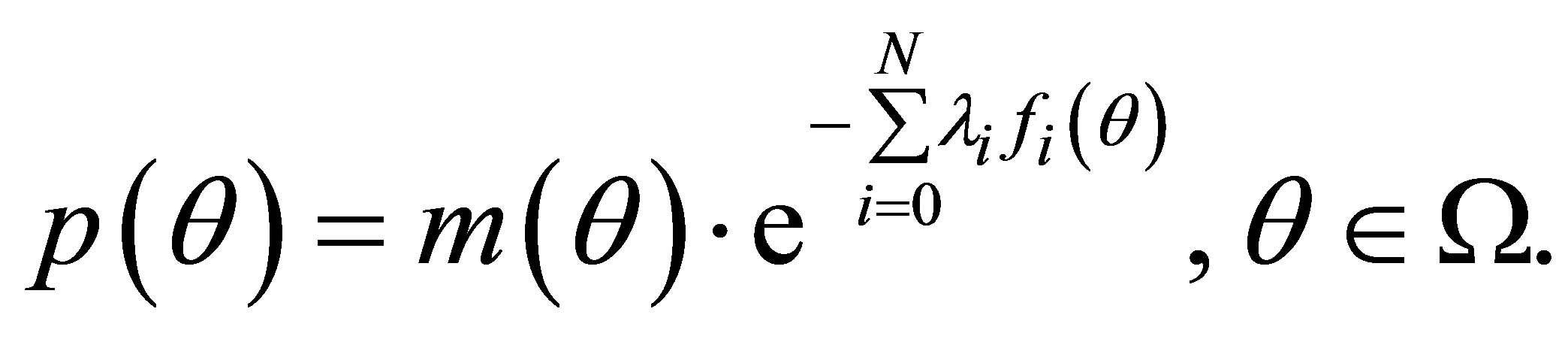 (1.8)
(1.8)
2.1. Testable Information
The PME solution (Equation (1.8)) does not specify the test functions . They are of major importance though since the solution is directly expressed in them. As stated in the introduction there is a convention of setting
 ,
,  etc. That is a habit, not a prescription. The choice of test functions must consequently be considered to be at our free disposal.
The difficulty or accuracy of estimating  is dependent on the explicit form of
 . Also, the information contained in the observation set
  is to a variable degree transferred to the estimate of
 . For instance, if
  all observations are equally weighted, but if
 ,
,
 (1.9)
(1.9)
the exponent  determines how much different observations contribute. In the asymptotic limit
 , the observation with the largest deviation is much more important than any other (which only contributes to the estimate of the mean). A lot of information is obviously disregarded. The estimator covariance will accordingly be large. Nevertheless, in many situations the range [6]
 is of much larger interest than any other information. The confidence interval is a more general statistic allowing for sample spaces without bound. From the perspective of objectivity, it thus appears difficult to prescribe any specific set
 , or even their number (N). Clearly, the larger amount of data or independent information that is available, the larger
  is allowed without resulting in unacceptable estimator quality, as expressed with its bias and covariance.
To illustrate how subjectivity enters in practice, assume we have gathered a set of prior observations  of a phenomenological constant
  contained in a computer model. To calibrate the model [8], i.e. determine the optimal values of its parameters and their uncertainties (
 being one of them) from observations, Bayesian estimation is applied. That requires complete prior information, i.e. knowledge of the prior pdf
 . Applying PME starting from
 , test functions
  must be selected. With the choice of
 , the partition function will according to Equation (1.5) read,
Since we are not aware of any ignorance, we set . The condition Equation (1.6) on
  implies,
A fair amount of subjective pragmatism now suggests  to be limited to even numbers and the support
  to extend to the whole real axis, since that allows us to determine
  with ease. The symmetry of the integrand then implies
 . If
. If  is prohibited,
 . The current assignment then translates into an approximation of the support
  as well as the factor
  of
of . The remaining Lagrange multiplier
  is obtained by re-scaling,
The resulting pdf,
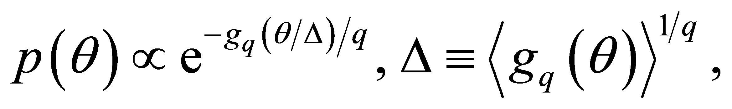 (1.10)
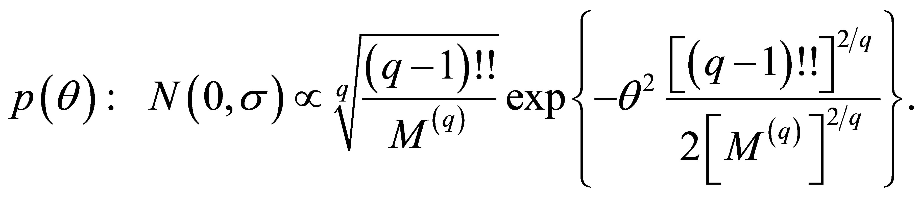
where  describes the
  order “width” of the pdf
 , is for different
  displayed in Figure 1. Clearly, the PME pdf is to a significant extent controlled by our subjective choice of test function, i.e.
 . The result varies between normal
  and uniform
 . More generally, with the understanding of the dependence on the test functions
  (Equation (1.8)), almost any PME pdf can be generated. It is only a matter of formulating the question (selecting
 ) to obtain the answer
  on virtually any desired form.
2.2. Quality of Estimation
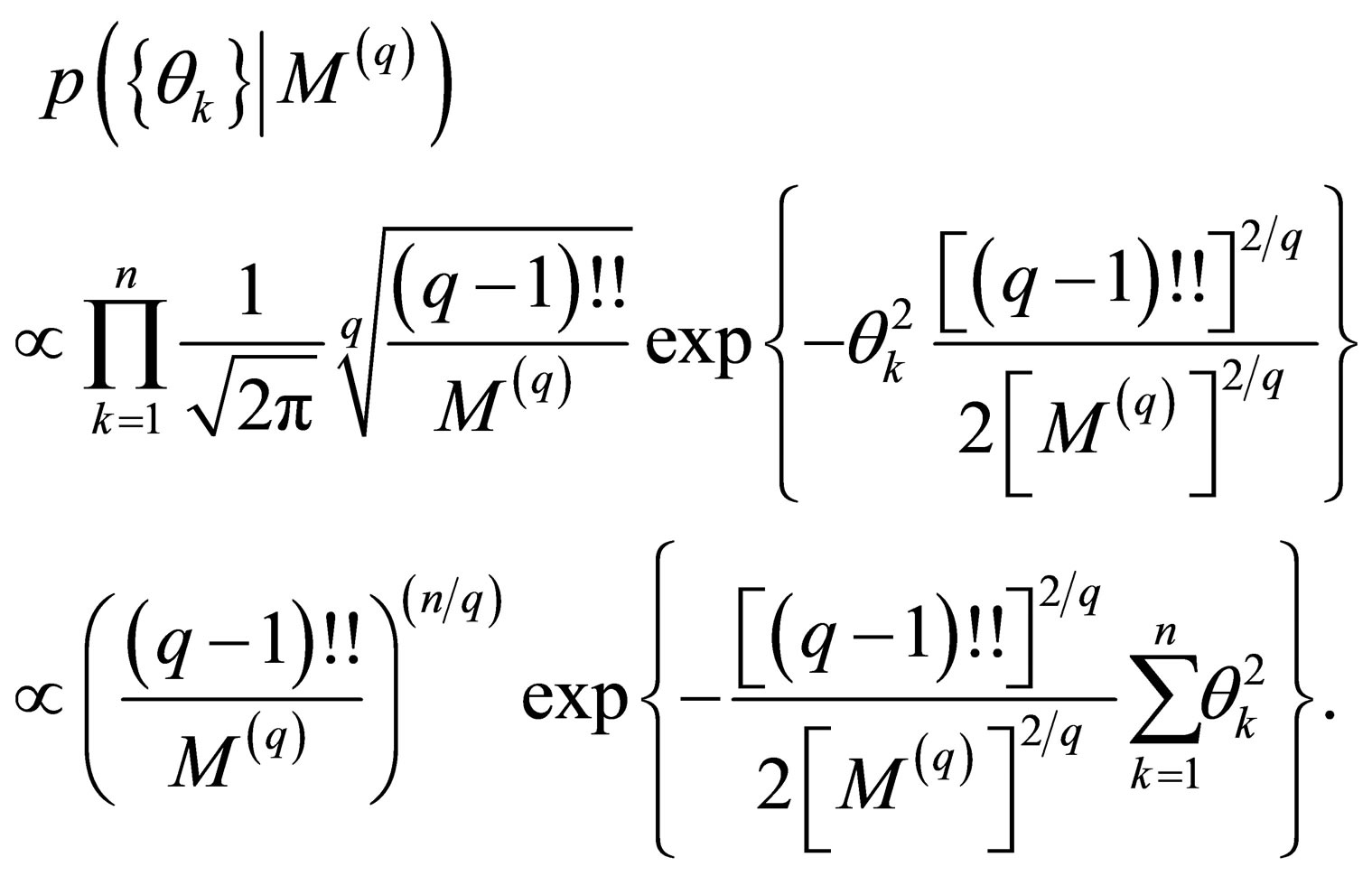
In practice, a testable piece of information  is estimated from raw observations with quality depending on the test function
 . The maximum entropy pdf
  can be directly formulated in our observations
 , using a specific estimator of the
  moment around the mean. An obvious estimator is given by,
 (1.11)
where  is an unknown constant which hopefully
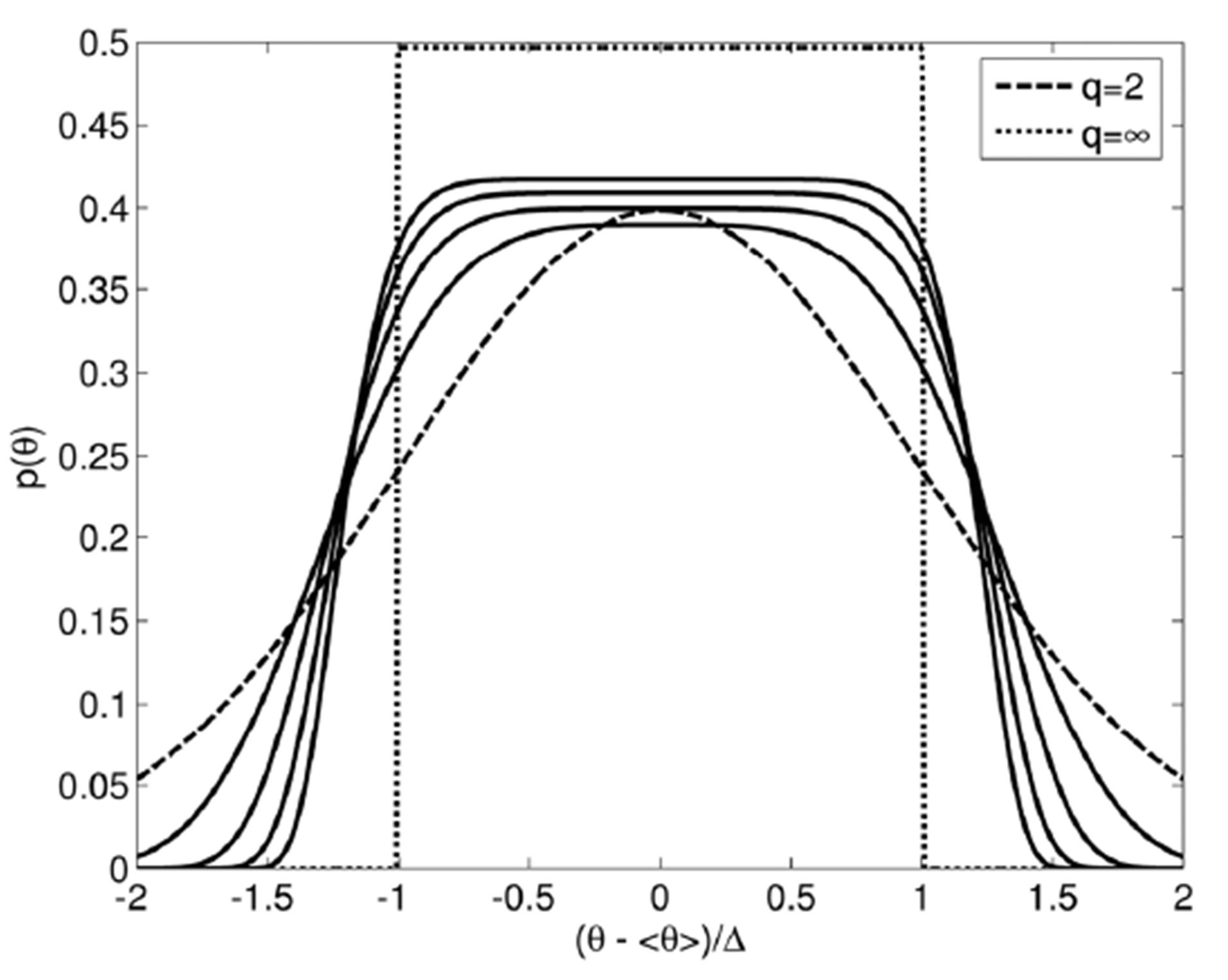
Figure 1. The maximum entropy pdf  for different kinds
  of testable information
 , see Equation (1.3). Case q corresponds to knowledge of the mean
  and the q-th statistical moment around the mean (
 , see Equation (1.9)).
can be selected to eliminate the bias, e.g. . To express the bias of
  in terms of
 , expand and calculate its expectation over observations
 ,
,
 (1.12)
On the other hand,
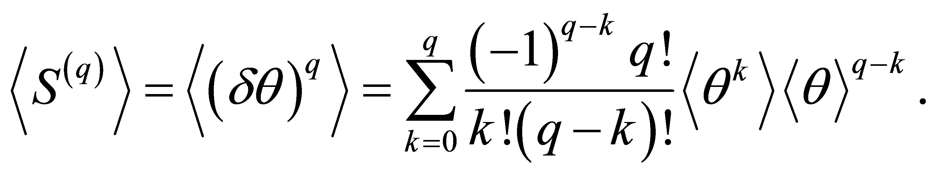 (1.13)
Clearly, the number of terms of  is much less than for
  for
for . Elimination of bias by proper selection of
  requires proportionality between
  and
and . That cannot in general be achieved since one of them have much more terms than the other. Thus, no scaling of
  can make it universally unbiased. Evaluating the first two coefficients of the expansion in Equation (1.12),
 (1.14)
Surprisingly, these two terms satisfies the proportionality required to eliminate the bias. Bias can thus be eliminated by rescaling up to , but not for
  (see estimation of kurtosis in [9]). This suggests the normalization,
 (1.15)
While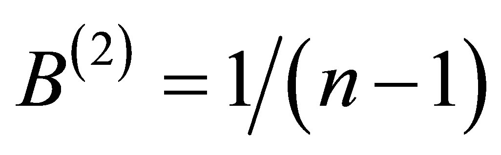 ,
, . Clearly,
  bears little resemblance to the conventional form
  of
of , where
  is the number of degrees of freedom.
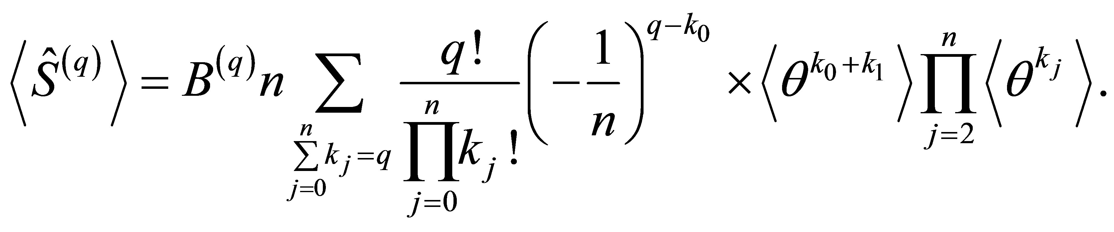
After failing to obtain an unbiased estimator of the  moment around an unknown mean, we may lower the ambition by assuming the mean
  is known. The corresponding estimator reads,
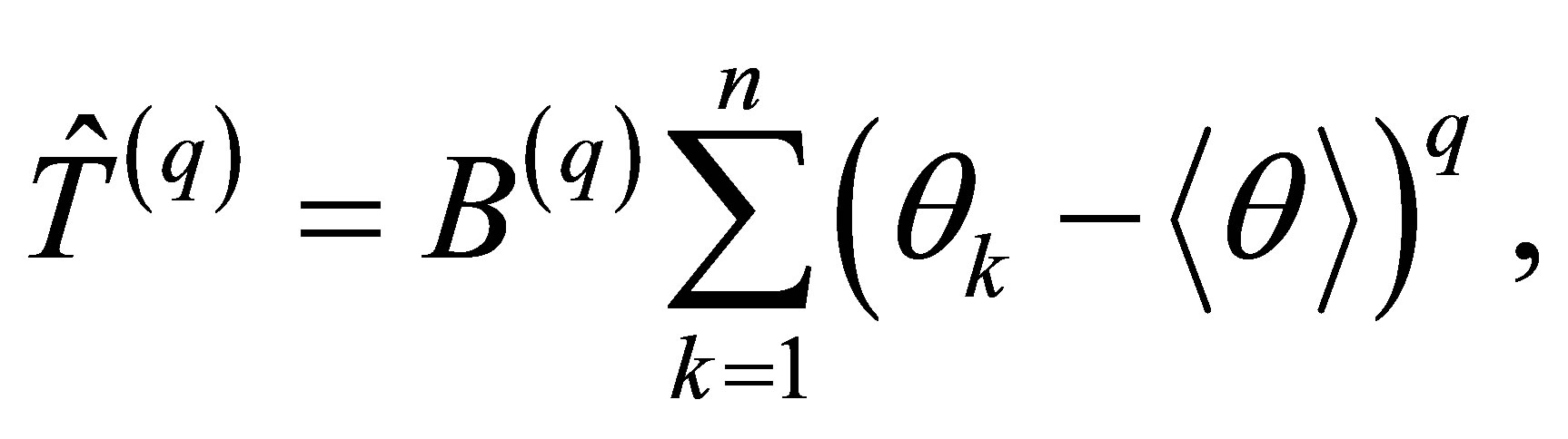 (1.16)
This is a considerably simpler situation for which the normalization 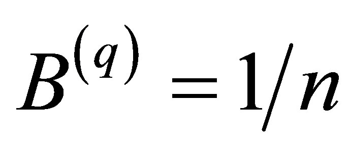 makes the estimator unbiased for all
 . The expected precision of any estimator
  describing its typical relative variation may be defined by,
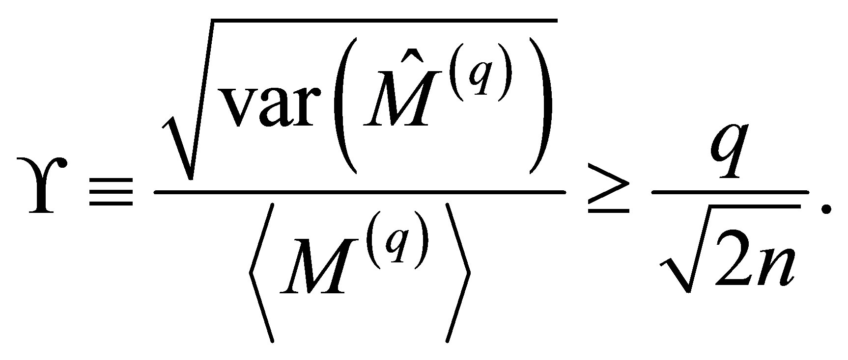
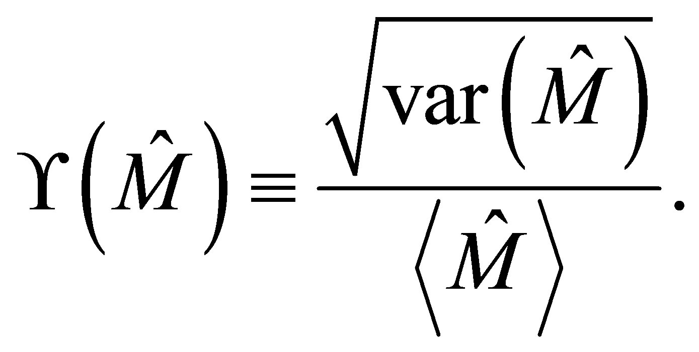 (1.17)
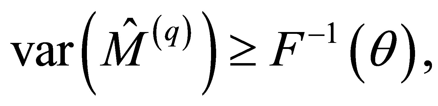
The least possible variance of any unbiased estimator  of
of  is given by the Cramer-Rao lower bound [2]
 , evaluated in Appendix A,
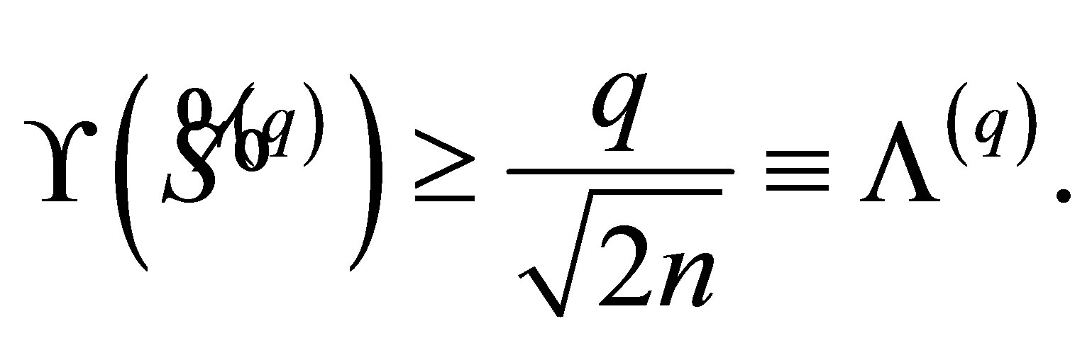 (1.18)
Since 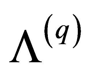 increases with
 , it is indeed more difficult to determine higher order moments accurately on an absolute scale, with any estimator. The efficiency
  of our specific estimator
  measures its relative quality,
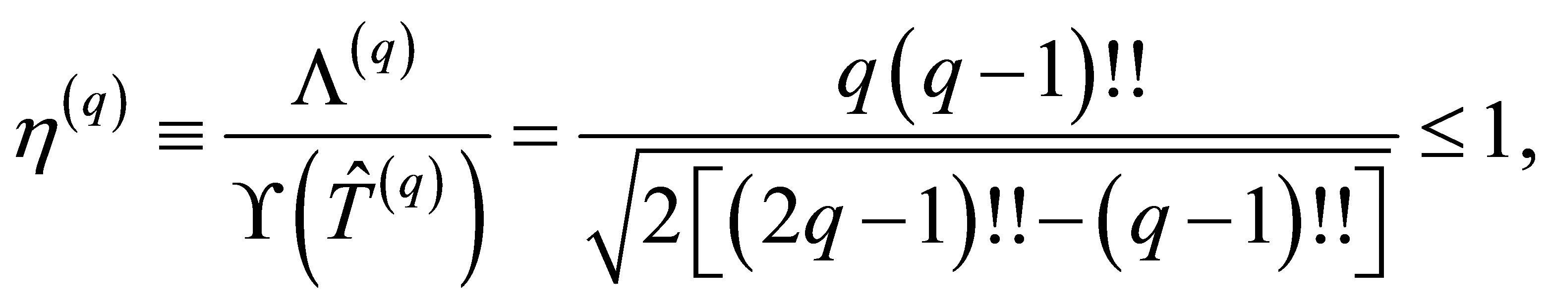 (1.19)
where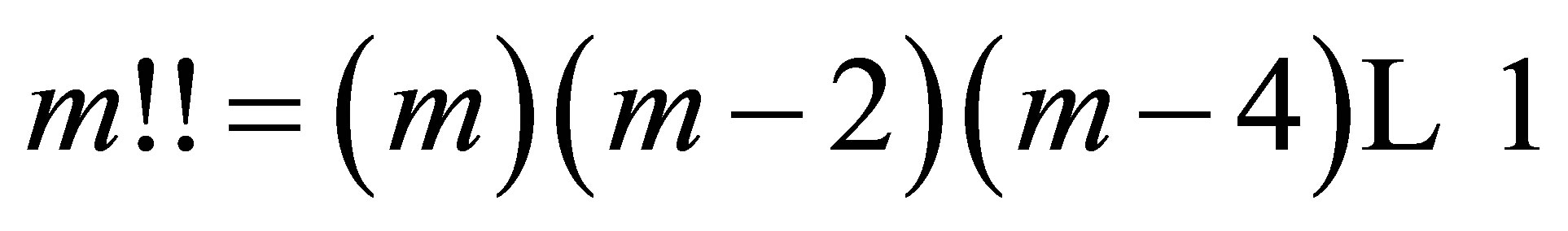 ,
,  is even and the precision
  is evaluated in Appendix B. For an efficient [2] estimator,
 . A low value of
  means that the potential for improvement of our estimator is large. Since
  decreases rapidly with
 ,
,  also becomes worse on a relative scale as
  increases. Nevertheless, the actual precision
  may or may not be satisfactory. The performance of the estimators
  is illustrated and compared to the Cramer-Rao lower bound in Figure 2, by evaluating their relative variation
  and bias
  numerically with multiple Monte Carlo ensembles.
To conclude, the determination of the PME pdf involved several subjective choices of processing the observations. The shape was here restricted by using monomial test functions . The order
  was limited to be even, to simplify the calculation of the integrals. Likewise, an infinite symmetric sample space
  was assigned. The difficulty of estimating various statistical moments around the mean increases rapidly with the order. If there are not more than a few samples it is in most cases impossible to reliably estimate any other moments than the first and the second. The application of PME thus relied upon rational selection rather than objective deduction.
2.3. Prior vs Posterior Application of PME
The PME constructs complete pdfs from incomplete testable information. It can be applied to the input (PME prior), or the output (PME post(-erior)) of the analysis. As no restriction or preference is stated in PME, both alternatives deserves to be considered and evaluated for efficiency and accuracy. The default method of linearization (LIN) [10] as well as the unscented Kalman filter (UKF) [11,12] and deterministic sampling (DS) [6]
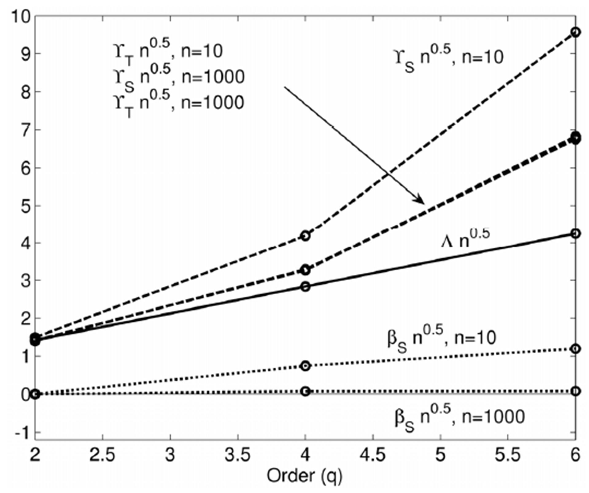
Figure 2. The relative precision  and
and  (dashed, Equation (1.17)) for the estimators
  (Equation (1.11)) and
  (Equation (1.16)), respectively, compared to the Cramer-Rao lower bound
  (solid, Equation (1.18)), for
  (connected by lines for clarity) and
  samples. The relative bias
  of
of  (dotted,
  given by Equation (1.15)) is also shown. The calculations were made for
  randomly generated samples of a normal distributed variable, equally split into ensembles of
  samples. Scaling with
  account for the main dependences on the number
  of samples (Equation (1.18)).
in general propagate statistics like covariance which later can be expanded to information related to entire pdfs, e.g. confidence intervals. That is, LIN, UKF, and DS promotes PME post. Monte Carlo simulations [13] or random sampling (RS) must start with complete statistical information to determine its random generator, i.e. RS requires PME prior.
An elementary example illustrates the principal differences between PME prior and PME post. Assume it is of interest to calculate the  confidence interval
  of an uncertain model
 , dependent on one parameter
 . Let the model uncertainty [8] be given by the mean
  and the variance
 . PME prior determines the input pdf
  to be normal distributed. Repeated generation of RS ensembles estimates their variation as function of their size: To achieve a standard deviation of the input
  confidence interval
  for
for  of about
 , no less than around
  randomly generated samples of
  are required. In RS, the model is evaluated for all these samples of
  and
and  is found by evaluating the results
 , ordering them, and extracting the
  percentiles. The known statistics
  and
and  can however be encoded exactly in no more than two(!) deterministic (calculated with a rule) samples
 . Assuming the model is close to linear-in-parameters, the model variance is mainly determined by the parameter variance, here represented by the parameter ensemble
 . In DS, the model variance is then with the argument of consistency given by the second moment around the mean of the model ensemble
 , i.e.
 .
.
Applying PME post to the result  and
and  implies that the resulting pdf is normal distributed, analogously to the input pdf in RS. That implies a coverage factor of
  resulting in a confidence interval,
 (1.20)
For estimating confidence intervals, PME does not in fact need to be utilized at all. By using another DS technique of ours, sampling on confidence boundaries [5], the desired interval can be found directly as,
 (1.21)
Consistency in evaluating confidence intervals of models here lead to the related concept of confidence boundaries in parameter space. For multivariate models with non-linear dependencies on parameters, both these results needs to be properly generalized [5,6]. Propagating a PME prior probability density function thus typically require several thousands of model samples [13,14] or complex algorithms [15]. The number of model samples propagated with DS for final completion with PME post can be as few as  for
for  parameters and increases with the known statistical information, the complexity of the model and acceptable accuracy of evaluation [16].
PME prior requires much more information to be analyzed, than PME post. For the example above, it means 3000 or 2 model evaluations. Plain rationality thus strongly favors PME post. The reason for requesting complete prior information is likely an ambition to find unique unquestionable answers, even if that in practice requires an extensive amount of blind assignments or assumptions. Unique is not equivalent to accurate however, and the quality of any assignment should be critically judged. The loss in efficiency of PME prior compared to PME post is not compensated by superior accuracy. In a number of cases, DS produces the correct result without any error: Any moment of any model given by a finite Taylor expansion can be exactly calculated with stratified DS [16]. Similarly, the confidence interval of any model  of any number (n) of parameters can be evaluated exactly [5], where
  are constants,
 all parameters, and
  is any non-linear monotonic function. For comparison, we are not aware of any general analytic method to propagate a univariate pdf determined by PME prior through any non-linear model. In this case, RS is a numerical method that yield arbitrarily small errors, but at very high computational cost. For “genuinely” multivariate problems RS seizes to be accurate. Multivariate refers to nontrivial finite dependencies of any order, as required for optimal modeling [16]. As far as we know, higher order dependencies (beyond second moments and not normal distributions) can only be implemented in RS by excluding samples. Exceptionally dense sampling is then required to accurately represent sampling density over the entire
  -dimensional sampling domain. Nevertheless, it is straight-forward to represent any arbitrary mixed moment in stratified DS [16]. The difficulty is just that the more requirements, the more samples are required. If not enough samples can be afforded it is possible to find the best approximating ensemble where different requirements are given different weights of importance. There are thus several reasons (as exemplified here) for PME post methods to not only be superior to PME prior approaches in efficiency, but also accuracy. The lean set of known input information in PME post is much simpler to analyze or propagate through any model than the complete information in PME prior.
With these observations, the traditional preference to prior instead of posterior completion of information with PME appears biased and strongly subjective. It is highly questionable if PME post methods like DS [6,11,16,17] can be claimed less accurate than state-of-the-art RS relying upon PME prior per se. As both practice statistical sampling once defined by Enrico Fermi [18], they are fully comparable. The choice is critical for complex models, as the low efficiency of RS easily render an impossible numerical task. Indeed, that is the main current obstacle for wide utilization of uncertainty quantification with RS.
Bayesian estimation is formulated for PME prior. The combination of the maximum likelihood function and the prior distribution makes Bayes approach superior to traditional approaches limited to the former. In practice though, two functions (PME prior) or two discrete sets of statistics (PME post) derived from observations are fused. Indeed, the common assumption of Gaussian noise and PME prior derived from the mean and covariance results in combination of covariance matrices (numbers) and not pdfs [8]. A non-trivial posterior distribution function requires non-Gaussian and/or correlated noise and utilization of no less than an infinite set of testable reliable information in the PME prior. If not so, Bayes estimation can without any loss of accuracy and relevance be made with PME post instead of PME prior, e.g. with DS instead of RS [8].
PME post (DS) makes it evident that results seldom are unique, while PME prior (RS) conceals ambiguities in more or less dubious or blind assignments in the problem set up. The indefiniteness of the result is an unavoidable consequence of starting with incomplete information, not the analysis. For PME post analyses (DS) this can easily be illustrated, for instance using different ensembles [6]. It is considerably more difficult for PME prior analyses (RS) due to their prohibiting numerical complexity. The contradictory consequence is that PME prior generally are considered more credible than PME post analyses, even if the latter are more honest and realistic as their flaws easily can be illustrated.
2.4. Towards Consistency and Rationality
The PME test functions should be selected according to the evaluation of the model, its behavior, and the quality of estimating the corresponding testable information. If we are interested in propagating the covariance of a signal processing model [6], we should consequently use a distribution which has been tested for representation of covariance. That is a consistent rather than an objective choice. Objectivity is an impossible target—selecting any method is a subjective choice. Our ignorance of  is rather reflecting relevance in perspective of our primary interest, or consistency throughout the analysis. It appears that consistency summarizes the goals of objectivity as well as our ignorance [1,3,4] and emphasizes the context. In contrast to objectivity, consistency expresses a relativity that can indeed be achieved in many situations, as well as measured, questioned and criticized.
The ubiquitous sparsity of statistical information in virtually all practical problems needs to be seriously addressed. If the realism of two approaches are comparable but their efficiency distinctively different, the choice should be based on rationality rather than consistency. Realism is distinct from resolution. Any complete set of assumptions will result in arbitrary high resolution, no matter how realistic the assumptions are. As the fidelity of the result never can be enhanced with blind assignments, it is questionable when statistical analyses should be made with distribution functions, rather than the testable information (statistics) these are derived from with PME. If desired, both approaches results in distribution functions. The completion of information is just made before (PME prior) or after (PME post) the analysis. The rational choice is PME post, as it propagates a minute fraction of the statistical information used in PME prior.
3. Conclusions
The character of maximum entropy (PME) distribution functions has been discussed. There are two principal innovations of our study. The PME solutions can to some extent be controlled by how primary data is processed. The prevailing preference for applying PME to the input (prior) and not the output (posterior) of statistical analyses is difficult to justify, as the their accuracy is comparable but the latter is computationally superior. The choice appears governed by the method of analysis. Hence, subjectivity enters into the processing of data as well how the analysis is made.
A non-trivial selection enters when observations are processed into testable information. A simple example illustrated common subjective choices, giving different results for identical observations.
Redirecting the focus from the treatment of known information to the targeted evaluation of the analysis emphasizes consistency, rather than objectivity. When consistency is indecisive, rationality or efficiency of the analysis provides obvious guidance. PME can be applied to find prior as well as posterior distributions. Its unconventional posterior application deserves to be seriously considered, as the analysis involves much less statistical information and is correspondingly more effective, than the prior. Consistency and rationality thus fundamentally questions the prevailing method of completing statistical information prior to the analysis, as in e.g. Monte Carlo simulations.
Maximal consistency and rationality are indeed primary goals of all our proposed methods of deterministic sampling. For complex models, such lean and customized approaches are often required to obtain any measure of modeling quality at all (within acceptable computational time). Without assessment of quality, any (modeling) result is of no value. These aspects are thus of paramount importance to our society where complex calculations (technical, physical, econometrical etc.) are rapidly increasing due to the fast development of computers.
REFERENCES
- D. S. Sivia and J. Skilling, “Data Analysis—A Bayesian Tutorial,” Oxford University Press, Oxford, 2006.
- S. M. Kay, “Fundamentals of Statistical Signal Processing, Estimation Theory,” Volume 1, Prentice Hall, Upper Saddle River, 1993.
- E. T. Jaynes, “Information Theory and Statistical Mechanics,” The Physical Review, Vol. 106, No. 4, 1957, pp. 620-630. http://dx.doi.org/10.1103/PhysRev.106.620
- C. E. Shannon, “A Mathematical Theory of Communication,” The Bell System Technical Journal, Vol. 27, No. 3, 1948, pp. 379-423.
- J. P. Hessling and T. Svensson, “Propagation of Uncertainty by Sampling on Confidence Boundaries,” International Journal for Uncertainty Quantification, Vol. 3, No. 5, 2013, pp. 421-444.
- J. P. Hessling, “Deterministic Sampling for Propagating Model Covariance,” SIAM/ASA Journal on Uncertainty Quantification, Vol. 1, No. 1, 2013, pp. 297-318.
- G. M. Ewing, “Calculus of Variations with Applications,” Dover, New York, 1985.
- J. P. Hessling, “Identification of Complex Models,” in Review, 2013.
- L. Råde and B. Westergren, “Mathematics Handbook,” 2 Edition, Studentlitteratur, Lund, 1990.
- ISO GUM, “Guide to the Expression of Uncertainty in Measurement,” Technical Report, International Organisation for Standardisation, Geneva, 1995.
- S. Julier and J. Uhlmann, “Unscented Filtering and Nonlinear Estimation,” Proceedings IEEE, Vol. 92, No. 3, 2004, pp. 401-422.
- S. Julier, J. Uhlmann and H. Durrant-Whyte, “A New Approach for Filtering Non-Linear Systems,” American Control Conference, Seattle, 21-23 June 1995, pp. 1628- 1632.
- R. Y. Rubenstein and D. P. Kroese, “Simulation and the Monte Carlo Method,” 2 Edition, John Wiley & Sons Inc., New York, 2007.
- J. C. Helton and F. J. Davis, “Latin Hypercube Sampling and the Propagation of Uncertainty in Analyses of Complex Systems,” Reliability Engineering and System Safety, Vol. 81, No. 1, 2003, pp. 23-69. http://dx.doi.org/10.1016/S0951-8320(03)00058-9
- T. Lovett, “Polynomial Chaos Simulation of Analog and Mixed-Signal Systems: Theory, Modeling Method, Application,” Lambert Academic Publishing, Saarbrücken, 2006.
- J. P. Hessling, “Stratified Deterministic Sampling of Multivariate Statistics,” in Preparation, 2013.
- J. P. Hessling, “Deterministic Sampling for Quantification of Modeling Uncertainty of Signals,” In: F. P. G. Márquez and N. Zaman, Eds., Digital Filters and Signal Processing, INTECH, Rijeka, 2012.
- N. Metropolis, “The Beginning of the Monte Carlo Method,” Los Alamos Science Special Issue, Vol. 15, 1987, pp. 125-130.
Appendix A Cramer-Rao Lower Bounds of Statistical Moments of a Normal Distributed Variable
Assume a random variable  with zero mean is normal distributed,
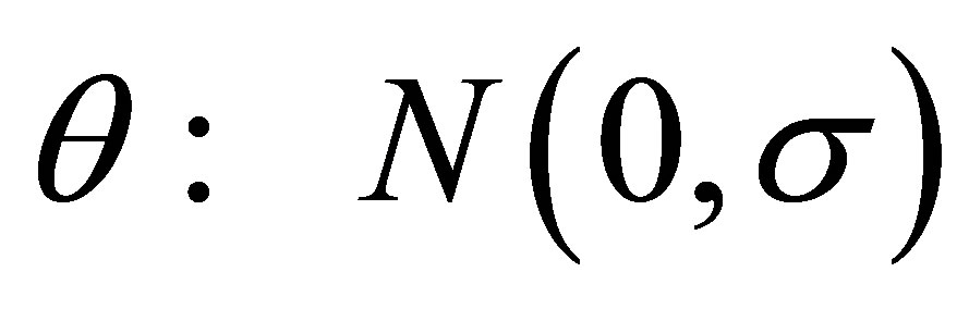 . By integrating by parts it can be shown that
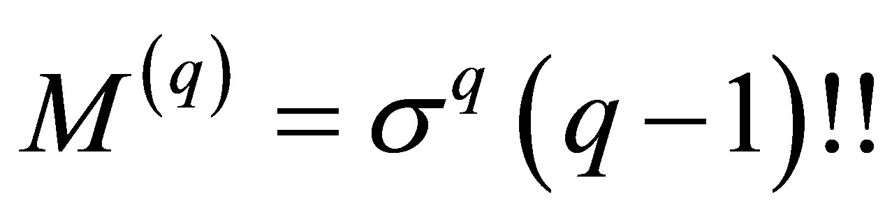 , where
 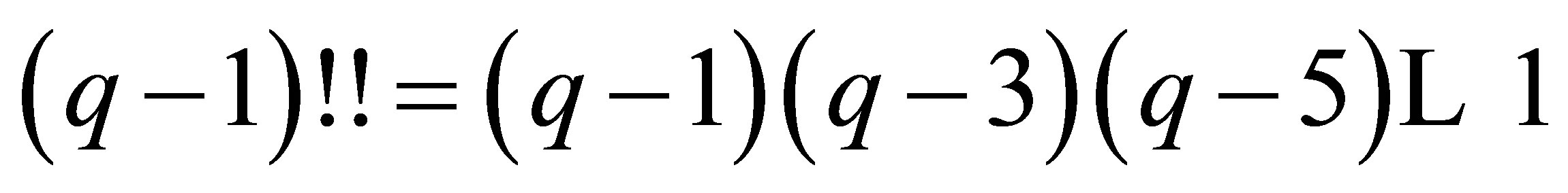 is the semi-factorial function. The probability distribution function for
  can then be expressed in
 ,
,
 (1.22)
For  independent observations
 , the likelihood function is given by,
 (1.23)
Cramer-Rao lower bound ([2]) now states that for any estimator  of
of ,
,
 (1.24)
where 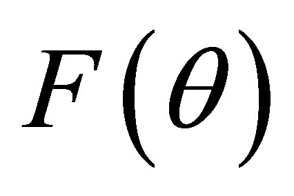 is the Fisher information matrix (scalar for one parameter),
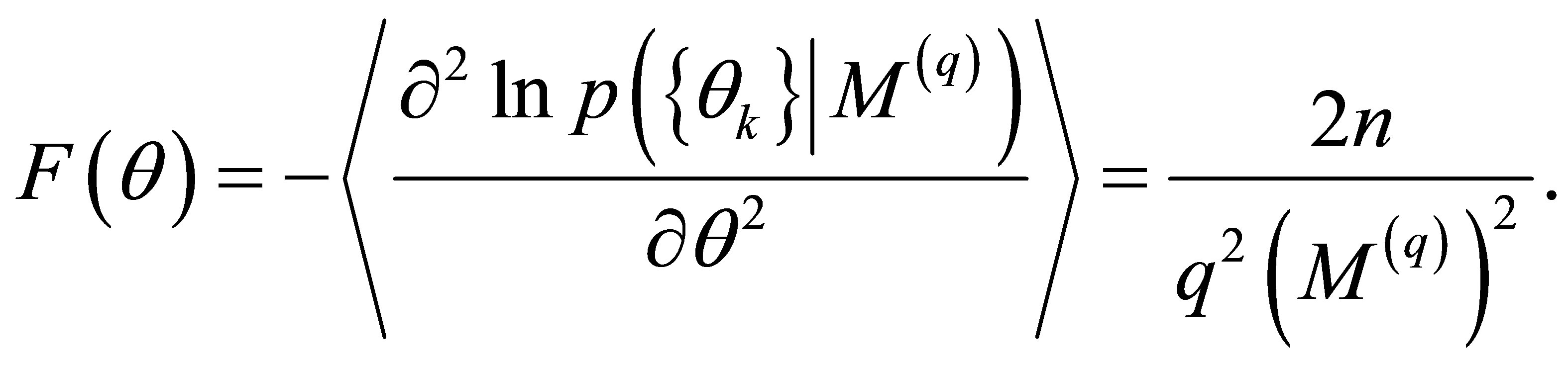 (1.25)
The expected precision  (Equation (1.17)) of the estimator
 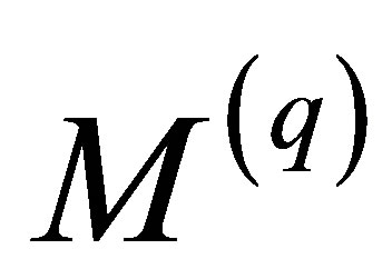 hence satisfies,
 (1.26)
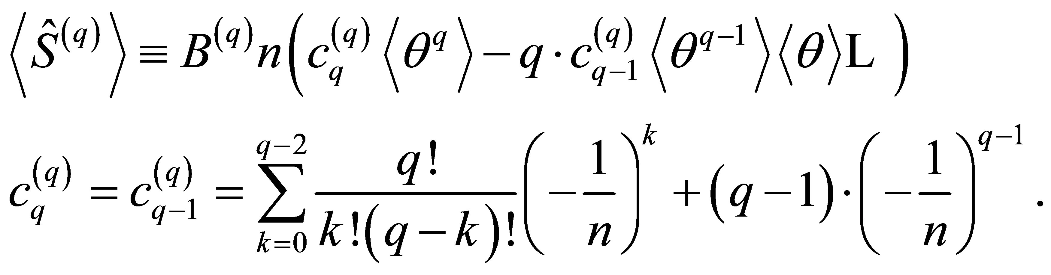
Appendix B Variance of Estimator of Statistical Moments around Given Mean
An estimator of the  statistical moment
 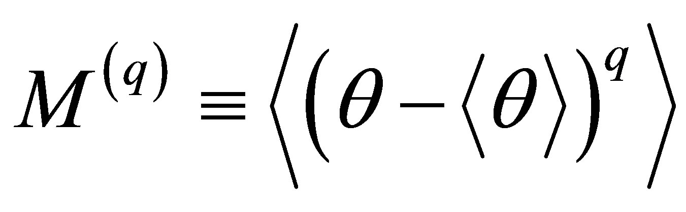 of
of  around a known mean
  from a set of
  independent observations
  is given by,
 (1.27)
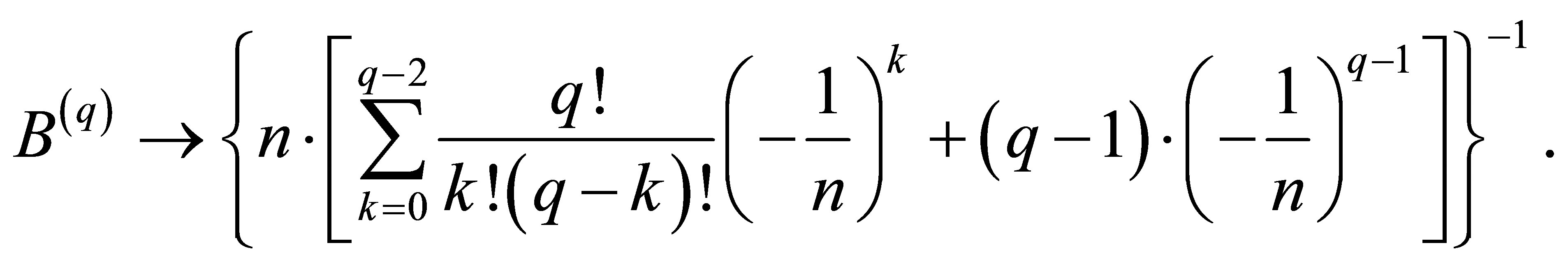
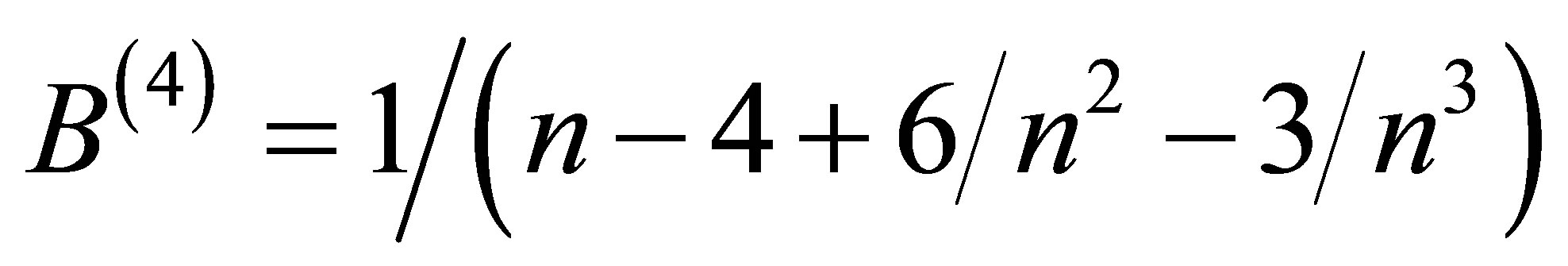
where the normalization constant B is chose to minimize its bias . Since
  is a known constant it is trivially found that
  eliminates all bias, for all values of
 . Its variance is found to be,
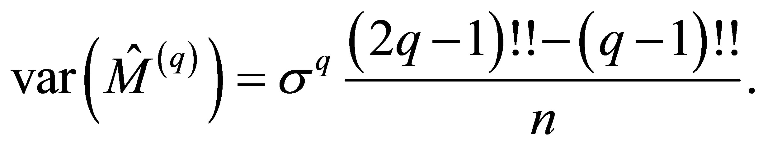
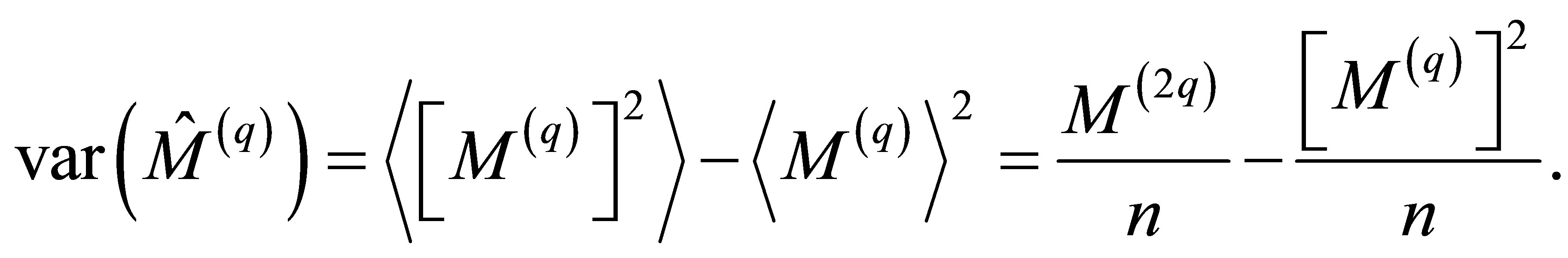 (1.28)
An explicitly value can be found for a normal distributed parameter, . Then, by recursively integrating by parts it is found that
 , where
  is the semifactorial function, giving
 (1.29)
NOTES
1Remark: “Ignorance” will here refer to the aspect of counting outcomes [1], not the concept of entropy [3].