Open Journal of Statistics
Vol. 3 No. 3 (2013) , Article ID: 32990 , 6 pages DOI:10.4236/ojs.2013.33018
Estimating Gini Coefficient Based on Hurun Report and Poverty Line
Department of Statistics and Finance, University of Science and Technology of China, Hefei, China
Email: zbfang@ ustc.edu.cn, zjp@ mail.ustc.edu.cn, daisydrj@ mail.ustc.edu.cn
Copyright © 2013 Zhaoben Fang et al. This is an open access article distributed under the Creative Commons Attribution License, which permits unrestricted use, distribution, and reproduction in any medium, provided the original work is properly cited.
Received February 28, 2013; revised March 29, 2013; accepted April 5, 2013
Keywords: Gini Coefficient; Quintile Rule; Curve-Fitting
ABSTRACT
Based on the review of various methods of estimating Gini coefficient, the paper applies a quintile rule to estimate Gini coefficient of rural areas, urban areas and the whole country using the grouped income data of urban and rural residents. Besides, the paper uses the curve-fitting method to roughly estimate Gini coefficient from eye-catching Hurun Rich List and the latest poverty line. The result shows that the estimation of Gini coefficient using quintile rule is small for both urban and rural area, while the value of the whole country is obviously larger, which is above the warning line of 0.4. It is indicated that the wealth gap mainly comes from the gap between urban and rural areas. On the other hand, the estimation of Gini coefficient using curve-fitting method is as large as more than 0.7, which implies that the wealth gap is highlighted from the analysis of the lowest and highest part of the wealth distribution. All in all, China’s current gap between the poor and the rich is serious. The reform of the income distribution needs to speed up to ensure social harmony and stability.
1. Introduction
The Italian statistician Gini first introduced inequality index in 1912 in [1]. The index was not designed for describing wealth disparities originally, but offered a statistic for depicting the dispersion of a random variable which was not related with the measure unit. Later, Dalton (1920) applied the index to study the problem of income distribution in [2], and the index was named Gini coefficient.
In the two-dimensional coordinate plane, where abscissa is the cumulative percentage of population and ordinate is the cumulative percentage of wealth, the curve formed by the scatter points is named as Lorenz curve as shown in Figure 1. If Lorenz curve is closer to the diagonal line, the distribution of wealth is closer to perfect equality; while if Lorenz curve is closer to the polygonal line, the distribution of wealth is closer to perfect inequality. Gini coefficient is the ratio of the area between perfect equality line and Lorenz curve to the area between perfect equality line and perfect inequality line.
The United Nations suggests Gini coefficient to reflect the gap between the wealthy and the poor (GBWP) following Table 1.
Usually, 0.4 is considered as the “picket line” of the income disparity. If Gini coefficient is above the “picket line”, polarization of wealthy and poor may easily cause the class antagonism and social unrest. The Gini coefficients of the main developed countries are between 0.24 and 0.36, and the United States’ is a little higher to 0.4.
China’s Gini coefficient was 0.412 in 2000, and the value climbed up to 0.465 in 2004 as reported by National Statistic Bureau (NSB). In June 2006, China Economic Weekly reported, “Our nation’s Gini coefficient is close to 0.5”. Since then, China’s Gini coefficient was not reported again. On 18th January, 2013, NSB released the Gini coefficients from 2003 to 2012, which were 0.479, 0.473, 0.485, 0.487, 0.484, 0.491, 0.490, 0.481, 0.477 and 0.474.
[3] borrowed Naffziger standard equation, and added two parameters considering Chinese realities, to calculate the Gini coefficients of 1980 and 1988, and they were 0.25 and 0.30. [4] estimated the Gini coefficients for 1993 and 1997, which were 0.375 and 0.39. [5] calculated the Gini coefficients of 1988 and 1995 based on the household sampling survey, and the values were 0.382 and 0.445. The study empirically analyzed Chinese income distribution from some aspects, and perfectly re-
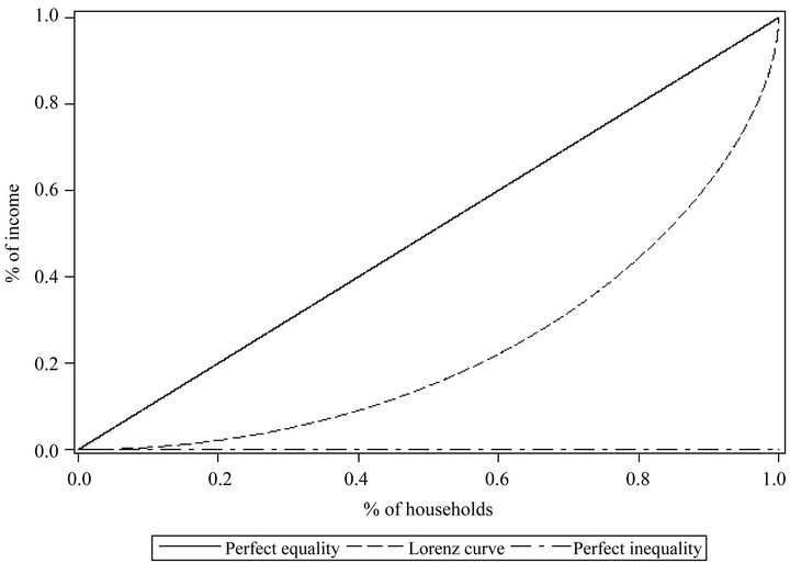
Figure 1. Lorenz curve.
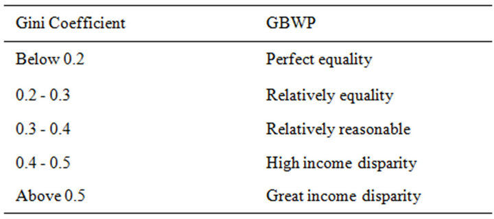
Table 1. Gini coefficient and GBWP.
vealed the degree and the trend of Chinese income-disparity. But they only calculate the coefficients for two years and did not give the calculating method in detail. China Household Finance Survey and Research Center of Southwestern University of Finance and Economics published a report “China Household Income Inequality Report”. The report showed that the Gini coefficient of household income was 0.61 in 2010, far above the global average value.
2. Review of the Estimation Methods of Gini Coefficient
Firstly, we review some estimation methods of Gini coefficient which have been used in practice.
2.1. Direct Calculation Method
Direct calculation method was mentioned when Gini introduced the inequality index, and he also offered specific algorithm which did not depend on Lorenz curve. It can directly measure the degree of income-disparity. The equation is as follows:
 (1)
(1)
where  is the absolute value of a pair of samples, n is the sample size and u is the average value of income.
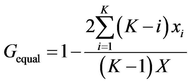
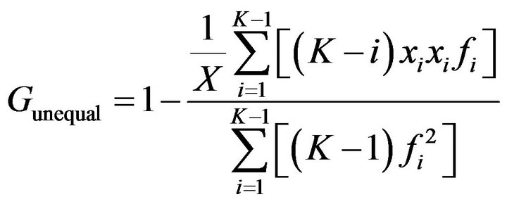
2.2. Grouping Method
[6] proposed a calculating method based on group data:
 (2)
(2)
 (3)
(3)
where X is the total wealth,  is the wealth of Group i,
  is the frequency of Group i. The two equations above are under the conditions of equal frequency group data and unequal frequency group data respectively.
2.3. Curve Fitting Method
As summarized in [7], by using some known points of Lorenz curve, Lorenz curve function  can be fitted, which is denoted as
 . Then, Gini coefficient can be integrated as follows:
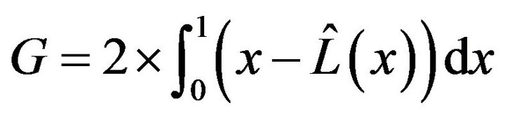 (4)
(4)
2.4. Distribution Function Method
Suppose a single resident’s wealth Y follows a distribution which has a probability density function . After estimating the unknown parameters of the distribution, Lorenz curve can be estimated using the following equation.
 (5)
(5)
Incorporating Equation (5) in Equation (4), and then the Gini coefficient can be determined.
The distribution function of the wealth has different forms in different scholars’ researches. [8] adopted general Beta distribution, [9,10] chose Pareto distribution, and [11] considered that log-normal distribution might be better.
2.5. Decomposition Method
Calculating Gini coefficient by decomposition method always depends on some known Gini coefficient values of separated groups. Hence, decomposition method is not an independent method for calculating the coefficient, but a method to decompose the coefficient and study the relationship among Gini coefficients of different groups.
[12] pointed out that Gini coefficient cannot be decomposed completely. Gini coefficient contains not only the intra-group differences, but also the inter-group differences and the interaction term. It can be expressed as follows:
 (6)
(6)
where G is Gini coefficient of the whole group,  is Gini coefficient of Group i,
  is the weight of
 ,
,  is the inter-group difference, and
  is the interaction term which indicates the overlapping of income distributions of different groups.
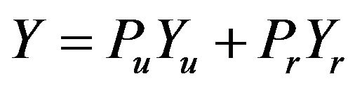
[13] introduced a decomposition method for Gini coefficient in his book—Income Distribution in Less Developed Counties.
 (7)
(7)
 (8)
(8)
where G is Gini coefficient of the whole group,  and
and  are Gini coefficients of urban and rural groups,
  and
and  are population proportions,
 ![]() and
and  are urban and rural average income per head. The implicit assumption of this method is that there is not overlapping of urban and rural income distribution. However, it cannot happen in actual situation, so there exist errors.
3. Two New Methods
Two new methods will be introduced in the rest part of the paper. And the methods mentioned above may be referenced in the new methods.
3.1. Quintile Rule Method
Firstly, Quintile Rule is introduced as in [14]: let f be a polynomial of degree not bigger than 5 such that
 and
and . Then

(9)
The formula derivation can be seen in [14]. Based on Quintile Rule, the calculation method will be explained for calculating Gini coefficient in 2010. The data used in this research is shown in Tables 2 and 3, which is extracted from China Statistical Yearbook published by NSB.
The population proportion of the five groups by income percentile can be considered approximately same. Thus, Quintile Rule method can be applied to calculating Gini coefficient. Let  be the function of Lorenz curve, the calculation process is summarized in Table 4.
Combining the equation  and Equation (9), Gini coefficient can be calculated.
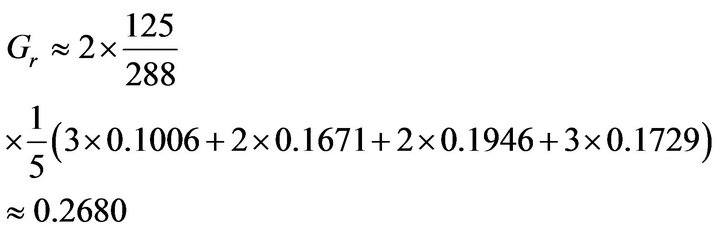
Gini coefficient of urban residents’ income:

Gini coefficient of rural residents’ income:
Then, in order to get the national Gini coefficient, decomposition method will be used. By referencing to [13], national Gini coefficient can be estimated based on Gini coefficients of urban and rural residents’ income.
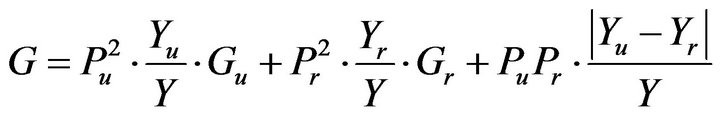 (10)
(10)
 (11)
(11)
where  and
and  are proportions of urban and rural population (49.95% and 50.05% in 2010),
  and
and  are urban and rural per capita annual income (19109.4 and 5919.0 yuan in 2010). Then the estimation of na

Table 2. Basic condition of urban households by income percentile (2010).
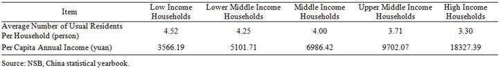
Table 3. Basic condition of rural households by income quintile (2010).
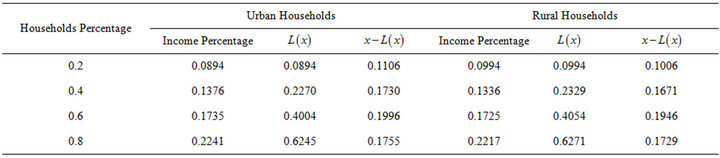
Table 4. Calculation process.
tional Gini coefficient in 2010 is 0.4015, obviously bigger than both of urban and rural Gini coefficients, which reflects the remarkable gap of wealth between urban and rural areas.
In the same way, Gini coefficients from 2003 to 2009 are also calculated presented in Table 5.
The results show that urban, rural and national Gini coefficients don’t fluctuate a lot recent years. National Gini coefficient even began to decline from 2006, which might be irreconcilable with people’s feeling. But the rural Gini coefficient is not far from the result of [15], so the estimation values are somewhat rational. The reasons why the values of Gini coefficients seem smaller than people’s feeling may be: firstly, the proportions of population in five groups are not equal exactly; secondly, the samples of urban and rural households are not representative, i.e. choosing specific samples artificially; lastly, the hypothetic function of Lorenz curve may be far different with the actual one. In spite of this, it can be seen from the smaller urban and rural Gini coefficients but bigger national value that the income gap between urban and rural residents are still big. Thus, it is urgent to promote farmers’ income to narrow the income gap.
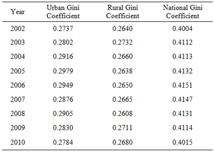
Table 5. Gini coefficient from 2002 to 2010 by quintile rule.
3.2. Estimation Method Based on Hurun Report and Poverty Line
Every year, regularly published Hurun Report is always attractable. When people surprise the rich’s great wealth, they should think about what the proportion of the total wealth the rich have actually. And the wealth gap can also be seen from them, so they have big contribution to national Gini coefficient. Therefore, we try to estimate Gini coefficient based on the Hurun Report, i.e. the rich and their wealth. The basic idea is estimating the proportion of the rich population and the proportion of their wealth, and then a point in the tail of Lorenz curve can be confirmed. In the same way, a point in the head can also be confirmed from the poverty line. According to various kinds of assumption about the forms of Lorenz curve, the function of Lorenz curve can be estimated, and then Gini coefficient will be calculated.
China Private Wealth Report 2010 published by Forbes showed that the private wealth of China had reached to 100 trillion yuan. About 383 thousand people had more than 10 million yuan for investing, which amounted to 22.4 trillion yuan. In Hurun Report, 1363 persons (about one millionth of the national population) held the wealth of 5.34 trillion yuan in 2010. At the end of 2010, the total population of China was 1.3409 billion (urban population was 669.78 million and rural population was 671.13 million). So, 0.02856% of the people had 22.4% of the wealth and 1.016 millionth of the people held 5.34% of the wealth.
On the other side, the standard of poverty alleviation in 2010 was 1274 yuan and the population under the standard was 26.88 million. Later, the new standard of poverty alleviation was 2300 yuan, and then the poverty population reached 128 million. Suppose that the standard of poverty alleviation was the maximum per capita income, it could be obtained that 2.0046% of the population possessed no more than 0.03425% of the wealth and more than 9.546% of the population held only 0.2944% of the wealth.
From the estimation above, four points of Lorenz curve can be roughly confirmed, which are (0.020046, 0.0003425), (0.09546, 0.002944), (0.9997144, 0.776), (0.999998984, 0.9466). Besides, it is sure that (0, 0), (1, 1) are also in Lorenz curve. Then, Lorenz curve can be fitted using these points. According to the estimation of the points, the actual Lorenz curve is under the fitting curve, and the actual Gini coefficient will also be larger than the value based on the fitting Lorenz curve.
The shape of Lorenz curve can be imagined from the above figure, and Gini coefficient may be large. In the following part, curve fitting method will be applied to estimate Gini coefficient.
Frequently-used curves include polynomial curve, exponential curve, power function curve, etc., and the quintile rule method can be seen as polynomial curve fitting in fact. As shown in Figure 1, Lorenz curve is increasing and convex to the below, and lies in the area constituted by diagonal line, X axis and . Therefore, it is supposed that Lorenz curve has the following function form.
 (12)
(12)
The unknown parameters  can be estimated using the data points in Figure 2.

Substitute the parameter estimations into Equation (12):
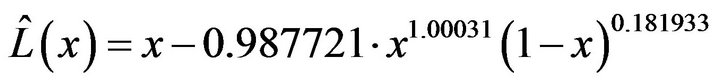 (13)
(13)
The fitting curve can be seen in the following figure.
It can be seen from Figure 3 that the curve fits the points very well. According to Equation (4), Gini coefficient of the fitting Lorenz curve can be calculated.
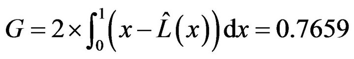
The actual Gini coefficient may be larger than 0.7659. China Household Finance Survey and Research Center of Southwestern University of Finance and Economics reported that Gini coefficient of household income was

Figure 2. Scatter diagram of lorenz curve.

Figure 3. Lorenz curve fitting.
0.61 in 2010, which was smaller than the estimation in this paper. It looks grandiloquent that Gini coefficient exceeds 0.7, while it may be not so large actually, or it might cause social unrest. Because we estimate the Gini coefficient based on the start part and the end part of the wealth distribution, it is unavoidably to overestimate the value. The estimation of Gini coefficient in the paper mainly reflects the great gap between two ends of the wealth distribution of China. Thus, the result only has academic significance. Although the estimation is rough, it indicates the huge gap between the rich and the poor in China, which is potentially harmful to sustainable development of economy and the social stability.
4. Conclusions
The paper reviews some kinds of frequently-used methods for estimating Gini coefficient, including direct calculation method, grouping method, curve fitting method, distribution function method and decomposition method. The urban, rural and national Gini coefficients from 2002 to 2010 are estimated by quintile rule based on the group data of urban and rural household income in NSB’s Statistical Yearbook. The results show that the urban and rural Gini coefficients are small, but the national Gini coefficients are significantly bigger, which implies that the gap between the rich and the poor mainly due to the gap between urban and rural areas.
In the second new method, some points in Lorenz curve are estimated firstly from Hurun Report and the poverty line. Then, curve fitting method is applied to estimated Lorenz curve and Gini coefficient. The result of estimated Gini coefficient is 0.76, which indicates the great gap between the rich and the poor. Although the actual Gini coefficient of China may not be so large, it still reflect the severity of the polarization between the rich and the poor. Therefore, after 18th CPC National Congress, the reform of income distribution should speed up, and the reasonable income distribution should be guaranteed when residents’ income doubles in the future, to make sure that the society is harmonious and stable.
REFERENCES
- C. Gini, “Italian: Variabilità e Mutabilità (Variability and Mutability),” In: E. Pizetti and T. Salvemini, Eds, Memorie di Metodologica Statistica, Libreria Eredi Virgilio Veschi, Rome, 1955.
- H. Dalton, “The Measure of the Inequality of Incomes,” The Economic Journal, Vol. 30, No. 119, 1920, pp. 348- 361. doi:10.2307/2223525
- Income Distribution Research Group of Nankai University, “Unfair Distribution of Income in China, Present Situation, Origination and Countermeasure,” Nankai Journal, No. 2, 1990, pp. 39-41.
- Research Office of the State Council, “Analysis and Proposition about Income Disparity of Urban Residents,” Economic Research Journal, No. 8, 1997. pp. 3-10.
- R. W. Zhao, S. Li and L. Carle, “Research on the Income Distribution in China,” China Financial and Economic Publishing House, Beijing, 1999.
- B. P. Nuria, “Approximation of Gini Index from Grouped Data,” Working Paper, 2003.
- Y. M. Wang, “Comparison of Calculation Methods of Gini Coefficient,” Statistics and Decision, No. 5, 2010, pp. 157-159.
- J. B. McDonald and Y. J. Xu, “A Generalization of the Beta Distribution with Application,” Journal of Econometrics, Vol. 69, No. 2, 1995, pp. 427-428. doi:10.1016/0304-4076(94)01680-X
- X. R. Chen, “Gini Coefficient and Estimation”, Statistical Research, No. 8, 2004, pp. 58-60.
- Q. Z. Chen and J. D. Chen, “A Note to the Lorenz Curve and Gini Coefficient,” Acta Scientiarum Naturalium Universitatis Pekinensis, Vol. 42, No. 5, 2006, pp. 613-619.
- B. W. Cheng, “Lorenz Curve and GINI Coefficient under Condition of Lognormal Distribution,” The Journal of Quantitative and Technical Economics, Vol. 22, No. 2, 2005, pp. 127-137.
- F. A. Cowell, “Measurement of Inequality,” In: A. Atkirrson and F. Bourguignon, Eds., Handbook of Income Distribution, North-Holland, Amsterdam, 2000.
- R. M. Sundrum, “Income Distribution in Less Developed Counties,” Routledge, London and New York, 1990. doi:10.4324/9780203168493
- L. Gerber, “A Quintile Rule for the Gini Coefficient,” Mathematics Magazine, Vol. 80, No. 2, 2007, pp. 133- 135.
- X. B. Qu and Y. Du, “The Regional Income Gap and Changes in Rural China during 1995 to 2008: Based on the Decomposition of Gini Index,” Economic Theory and Business Management, No. 7, 2010, pp. 74-80.