Open Journal of Statistics
Vol.3 No.2(2013), Article ID:29809,10 pages DOI:10.4236/ojs.2013.32008
New Tests for Assessing Non-Inferiority and Equivalence from Survival Data
United States Food and Drug Administration, Silver Spring, USA
Email: Kallappa.Koti@fda.hhs.gov
Copyright © 2013 Kallappa M. Koti. This is an open access article distributed under the Creative Commons Attribution License, which permits unrestricted use, distribution, and reproduction in any medium, provided the original work is properly cited.
Received October 5, 2012; revised November 10, 2012; accepted November 20, 2012
Keywords: Right-Censored Data; Kaplan-Meier Estimate; Bootstrap Standard Error; Generic Drugs
ABSTRACT
We propose a new nonparametric method for assessing non-inferiority of an experimental therapy compared to a standard of care. The ratio  of true median survival times is the parameter of interest. This is of considerable interest in clinical trials of generic drugs. We think of the ratio
  of the sample medians as a point estimate of the ratio
 . We use the Fieller-Hinkley distribution of the ratio of two normally distributed random variables to derive an unbiased level-α test of inferiority null hypothesis, which is stated in terms of the ratio
  and a pre-specified fixed non-inferiority margin δ. We also explain how to assess equivalence and non-inferiority using bootstrap equivalent confidence intervals on the ratio
 . The proposed new test does not require the censoring distributions for the two arms to be equal and it does not require the hazard rates to be proportional. If the proportional hazards assumption holds good, the proposed new test is more attractive. We also discuss sample size determination. We claim that our test procedure is simple and attains adequate power for moderate sample sizes. We extend the proposed test procedure to stratified analysis. We propose a “two one-sided tests” approach for assessing equivalence.
1. Introduction
Non-inferiority and equivalence trials aim to show that the experimental therapy is not clinically worse than (non-inferiority) or clinically similar to (equivalence) an active control therapy. As the statistical formulation is one-sided, non-inferiority trials are also called one-sided equivalence trials. ICH E10 [1] is an authentic and official guidance document on the choice controls in noninferiority clinical trials. The active control, which is also called a reference, is usually a standard of care. As noted in [1], most active-control equivalence trials are really non-inferiority trials intended to establish the efficacy of a new therapy. A non-inferiority trial is conducted to evaluate the efficacy of an experimental therapy compared to an active control when it is hypothesized that the experimental therapy may not be superior to a proven effective therapy, but is clinically and statistically not inferior in effectiveness. If the experimental therapy has a better safety profile, and/or easier to administer, and/or costs less, then non-inferiority trials are considered appropriate [2].
Confidence intervals on hazard ratios are used to assess equivalence and non-inferiority from survival data. The concept of hazard ratio is elusive. Clinicians find it hard to understand. Koch [3] says that though it is straightforward to construct confidence intervals on hazard ratios, it can be awkward to interpret. Wellek [4] proposed a log-rank test for equivalence of two survivor functions. According to Wellek, the survivor functions are considered equivalent if the absolute difference between the two survival curves is less than a pre-specified margin  over the whole range of values of event-time. His test is carried out in terms of the regression coefficient for a dummy covariate indexing the trial arms. Though Wellek’s paper is remarkable in its technical content, the test procedure is not used in practice. A possible reason is that his definition of equivalence criterion is conceptually difficult for clinicians to understand. Moreover, this formulation of the problem requires that the survival curves belong to the same proportional hazards model. The proportional hazards assumption is often inappropriate. We would like to point out that if the proportional hazards assumption holds good, the tests for non-inferiority (and equivalence) in terms of medians would be more attractive.
Because the distribution of survival times tends to be positively skewed, the median is the preferred summary measure of the location of the distribution. Also, the median is straightforwardly informative to the clinicians. Efron [5] said it very nicely—“The median is often favored as a location estimate in censored data problems because, in addition to its usual advantage of easy interpretability, it least depends upon the right tail of the Kaplan-Meier curve, which can be highly unstable if censoring is heavy.” Simon [6] emphasizes the importance of confidence intervals on median survival times. He writes: “For exponential survival distributions, the hazard ratio equals the ratio of medians. Exponential survival means that the survival curve is a straight line on a semilogarithmic scale (log survival probability over time). Because exponential distributions are good approximations to the survival curves seen in many kinds of advanced cancer, confidence intervals for the hazard ratio are often interpreted as confidence intervals for the ratio of medians.” Simon also explains how to calculate a confidence interval on the ratio of median survivals when the survival distributions are exponential. As a result, it has become a common practice in clinical trial study reporting to give point and interval estimates for the median survival time. This motivated us to consider testing for equivalence and non-inferiority of an experimental therapy compared to a reference therapy in terms of their median survival times. As assessing non-inferiority in terms of the difference between median survival times is trivial, we focus on their ratio.
Rubinstein et al. [7] were probably the first to consider the problem of testing the null hypothesis that the median survival times are equal against an alternative that the median survival time for the experimental treatment exceeds that of the control arm. They assumed exponential distributions for survival data. Britsol [8] presents a modification to Rubinstein’s procedure for situations where it is desired to show that the experimental treatment is not much worse than the control. As noted by Berger and Hsu [9], and Hauschke and Hothorn [10], testing for non-inferiority in terms of the ratio of the averages often reflects clinical rationale rather than the difference between the averages. Bristol wants to test the null hypothesis that the ratio of medians is less than or equal to a fixed margin ![]() against the alternative that the ratio exceeds
against the alternative that the ratio exceeds![]() . To simplify the matter, he assumes that failure times have exponential distributions. Bristol’s real interest is in testing the ratio hypothesis
. To simplify the matter, he assumes that failure times have exponential distributions. Bristol’s real interest is in testing the ratio hypothesis  stated in (3.1) below in Section 3. However, he uses log transformation of the ratio to derive an asymptotic test. We circumvent this problem by introducing the Fieller-Hinkley (hereafter abbreviated as F-H) distribution on the ratio of two normally distributed random variables. Moreover, we don’t assume failure times to follow exponential or some other parametric distributions.
2. One Sample Survival Model, Median Estimate and Standard Error
We develop the tests under the frame work of a randomly right-censored survival model. We assume that
 are iid random variables with a continuous distribution function F, and that F has a density f and median
 . These variables represent the event-times of the subjects under observation. Associated with each
 ![]() is an independent censoring variable
is an independent censoring variable , which are assumed to be iid from a censoring distribution
 . The data consist of
 ![]() pairs
pairs , where
 ![]() is either an observed failure-time
is either an observed failure-time ![]() or an observed censoring time
or an observed censoring time , and
, and . The basic quantity employed to describe time-to-event phenomenon is the survivor function
 . The median survival time estimate is given by
 , where
is the product-limit estimate of . That is, the median survival time is estimated from the product-limit estimate to be the first time that the survival curve falls to 0.5 or below. The sample median
 ![]() is asymptotically normally distributed with mean
is asymptotically normally distributed with mean . The variance
  of
of ![]() is mathematically intractable. The SAS lifetest procedure provides an estimate of survivor function accompanied by survival standard error [11]. By default, the SAS lifetest procedure uses the Kaplan-Meier method. It also produces a point estimate of the median
is mathematically intractable. The SAS lifetest procedure provides an estimate of survivor function accompanied by survival standard error [11]. By default, the SAS lifetest procedure uses the Kaplan-Meier method. It also produces a point estimate of the median  of
of  and the 95% confidence interval-derived by Brookmeyer and Crowley [12]. Brookmeyer and Crowley obtained the confidence intervals by inverting a generalization of the sign test for censored data. They did not need the standard error of the sample median. Obviously, the SAS lifetest procedure does not provide the standard error of the sample median
![]() . One form of the asymptotic variance of median
. One form of the asymptotic variance of median ![]() is
is
 , (2.1)
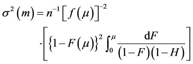
where  is found using the Greenwood’s formula [13]. A slightly different version of
  is provided in [14]:
 (2.2)
(2.2)
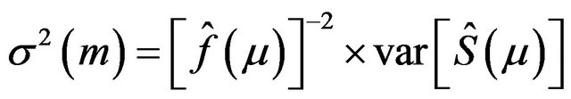
As f is unknown, the variance  given either in (2.1) or (2.2) becomes useless in estimating the population median time
  [15]. We propose to estimate the standard error of
 ![]() using the Efron’s bootstrap [5], which does not make any distributional assumptions. In a single sample setting, Efron’s bootstrap may be described as follows. We draw a bootstrap sample
using the Efron’s bootstrap [5], which does not make any distributional assumptions. In a single sample setting, Efron’s bootstrap may be described as follows. We draw a bootstrap sample 
 by independent sampling
 ![]() times with replacement from F and calculate the median
times with replacement from F and calculate the median
 . We repeat this independently B times, obtaining
  medians:
 . An estimated variance of the sample median time
 ![]() is
is
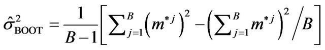 (2.3)
(2.3)
One may set  equal to 1000. This is called “modelfree” or the Efron’s bootstrap procedure II. The University of Texas at Austin [16] has provided some introductory SAS codes needed to resample a SAS dataset.
Efron [5] states: the bootstrap estimate  given in (2.3) is a consistent estimate, but
 ![]() in (2.1) or in (2.2) itself may be meaningless. Therefore, we assume that
in (2.1) or in (2.2) itself may be meaningless. Therefore, we assume that , which does not depend on either f or
  is a viable substitute for
 . Thus, we work under the notion that the sample median time
 ![]() is asymptotically normally distributed with mean
is asymptotically normally distributed with mean  and variance
 . We suppress the subscript BOOT of the estimated variance in (2.3). In fact, Keaney and Wei [17], among others, have used bootstrap to find the standard error of
![]() .
.
What is an indication of an unstable median or heavy censoring is a crucial question. As observed in [12], if the survival curve is relatively flat in the neighborhood of 50% survival, there can be great deal of variability in the estimated median. It would be more appropriate to cite a confidence interval for the median. We propose a simple rule of thumb. If the upper limit of a 95% confidence interval on median is not available, one may conclude that median is unstable and/or censoring is heavy. Therefore, the proposed tests should work efficiently when the Brookmeyer-Crowley upper limit of a 95% confidence interval on median is available. This also minimizes the number of bootstrap samples whose Kaplan-Meier curves do not reach 0.5 survival probability. In addition, asymptotic normality requires that .
.
3. Null and Alternative Hypotheses
Let  and
and  denote the times to event for the experimental and reference treatment groups, respectively. We use
  and
and  to denote the survival functions, and
  and
and  to denote the medians of
  and
and , respectively. Depending on the application one may test
 (3.1)
(3.1)
Here  and large median values point to large positive effects. For example, the null and alternative hypotheses in (3.1) are appropriate if non-inferiority as measured by the overall survival of patients is desired. In some other applications, small median values may point to large positive effects, in which case, for proving noninferiority, one may test
 (3.2)
(3.2)
where . For example, if duration of anemia (or time to response) is the clinical endpoint, it is appropriate to consider the null and alternative hypotheses in (3.2). Here
  and
and  indicate that the experimental therapy is not inferior to the reference therapy. The lower and upper bounds
  and
and  defining non-inferiority are called non-inferiority margins. The selection of noninferiority margin
  (or
(or ) depends upon a combination of statistical reasoning and clinical judgment. For a discussion on the choice of a non-inferiority margin, reference is made to ICH-E10 document [1]. For example, testing
 (3.3)
(3.3)
is of considerable interest in clinical trials of generic drugs. Henceforth, we assume that two independent sample  of possibly right-censored event-times are given. We use
  to represent the data. The sample size
  and
and  are sufficiently large. The censoring proportion, in each arm, is moderate. That is, the trial is designed to have long enough follow-up time so that more than one half of the subjects in both arms had the event. Let
  and
and  denote the product-limit survival estimates and
  and
and  denote the median time estimates for the experimental and reference groups, respectively. The sample medians
  and
and  are independently asymptotically normally distributed with means
  and
and , and variances
  and
and , respectively. As mentioned in Section 2, we assume that the bootstrap variances
  and
and  given by (2.3) are the de facto variances of
  and
and , respectively. The proportional hazards assumption is not required. However, we assume that the each treatment group has survival curve that is not relatively flat in the neighborhood of 50 percent survival. We also assume that each median estimate is at least two times larger than its standard error. Then the ratio
  follows the F-H distribution that is briefly described in the next section.
4. Fieller-Hinkley Distribution
Let  and
and  be normally distributed random variables with means
![]() , variances
, variances  and correlation coefficient
 . Let
. Let . Fieller [18] obtains the probability density function
  of W. Hinkley [19] derives the cumulative distribution function
  of
of . We have not shown
  and
and 
here due to lack of space. As a special case, Hinkley has shown that as  that is, as
 ,
,
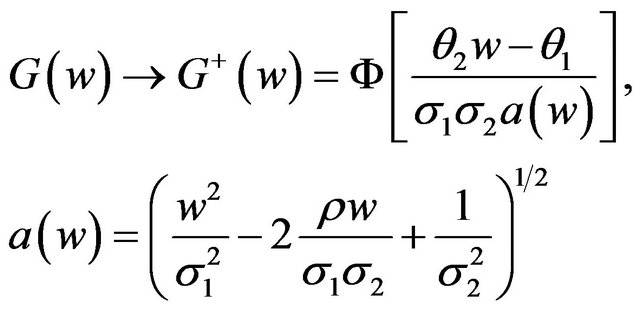 (4.1)
(4.1)
where  denotes the standard normal distribution function. In what follows, we consider the case where
  and
and  are statistically independent, and therefore, we set
 . Note that the argument in
  may be written as
 , where
 . The probability density function corresponding to
 , when
 , is
, is
 where
where  denotes the standard normal density function.
The distribution  is unimodal but not necessarily symmetric. It has a median equal to
 . The superscript
 ![]() in
in  refers to
  being a positive valued random variable. As the ratio of median survival times is always positive, we suppress the superscript.
Koti used the F-H distribution to derive non-inferiority tests under analysis of variance setting [20]. Koti also used the F-H distribution to derive tests for null hypothesis of non-unity ratio of proportions [21]. In this paper, his test procedure is extended to survival data analysis. We think of the ratio  as a point estimate of the ratio
  and we intend to use the distribution G of the ratio W to make inference on
 . As usual,
  denotes an observed value of
 . We regard the variances
  and
and  as nuisance parameters. In what follows, we replace
  and
and  by their bootstrap estimates
  and
and , respectively.
5. Test for the Lower Inequality
In this section we consider testing the null hypothesis  against the alternative hypothesis
 , which are stated in (3.1). Under the null hypothesis
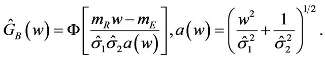
 , the distribution function of
 , the ratio of sample medians, is given by
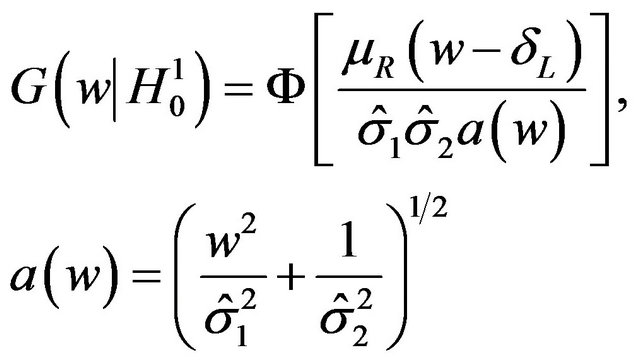 (5.1)
(5.1)
Intuitively,  should be rejected in favor of
  for large observed values of
 . We reject
  in favor of
  if
if , where
 .
.
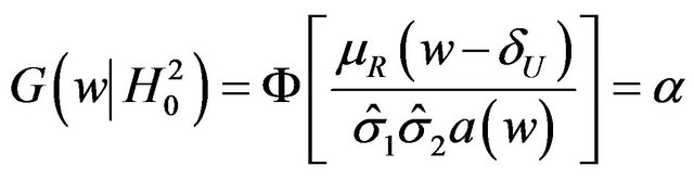
We need to find a cutoff point  that satisfies the equation
 (5.2)
(5.2)
where  is the 100a-th percentile of the standard normal distribution. The cutoff point
  satisfying (5.2) defines the rejection region for a given value of
 . Note that
  is the median of
  for all
  and the cutoff point
  for
for . To construct a test that has a significance level less than or equal to
 ![]() for all
for all , we proceed as follows. Calculate
  percent confidence intervals on
  and
and , where
 . Let
. Let  and
and  denote these confidence intervals on
  and
and , respectively. These confidence intervals should be as wide as possible. Let
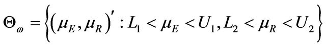 (5.3)
(5.3)
We describe  in (5.3) as a rectangular parameter space. Let
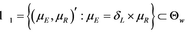 , and
, and
 denote the domain of the line
 . Here
  represents the parameter space under the simple null hypothesis
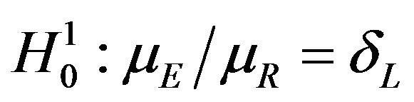 . We assume that
  is nonempty.
Consider  where both
  and
and  are in
  and satisfy (5.2) for some
  and
and . That is,
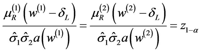 and
and . It means that
 .
.
Now  increases as w increases.
This implies that  and
and
Therefore,
 , and
, and
 (5.4)
(5.4)
This is graphically illustrated in Figure 1. Two F-H distribution functions with  are shown in Figure 1. The graph in solid line represents
  with
with  and the other one represents
  with
with . Here we have used
 , and
, and
 . Note that in the upper half portion of Figure 1, the distribution function
  runs below the distribution function
 . That is, for each x-coordinate
 , the y-coordinate for
  with
with  is lower than the one for
 .
.
This is what is claimed in (5.4). The reader may note that , and
, and
 That is,
 and
and
 .
.
Let  denote the smallest
  in
in  and
and
 . Then from (5.4), it follows that
 defines the critical region. That is, reject
  if
if . The significance level
 is less than or equal to
 ![]() for all
for all
 . Therefore, the rule that rejects
  for
for
 is a level
 ![]() test.
test.
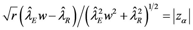
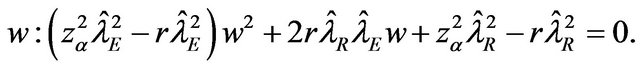
The cut off point  can be determined as follows. Square both sides of Equation (5.2) with
  replaced by
  and get a quadratic equation:
 , where
 and
and
 .
.
The roots of the quadratic equation are
 . The root that is smaller than
  defines the critical region of the test. Alternatively, one may use the SAS PROBNORM for tabulating
  and find
 .
.
5.1. p-Value and Power of the Test
The p-value for the test is
 (5.5)
(5.5)
where  is the observed ratio. The power of the proposed test is the probability that the null hypothesis
 , will be rejected when the alternative hypothesis
 , is true. We define the power function
  for a given alternative
  as
as
 (5.6)
(5.6)
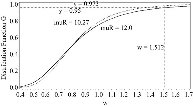
Figure 1. Two DFs of W both with a median of 0.8.
Usually, in designing a clinical trial, one aims to have a power over 0.5. Note that the power, for example,  in (5.6) exceeds 0.5 only if
 . For a given
 , it readily follows that
  for all
 . Therefore, the power
  may be called the minimum power.
5.2. The Test Is Unbiased
Note that
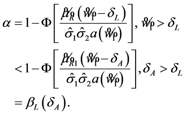
That is, the type-I error probability is at most ![]() and the power of the test is at least
and the power of the test is at least![]() . Thus, the test is unbiased.
. Thus, the test is unbiased.
6. Test for the Upper Inequality
Next, we discuss testing the null hypothesis  against the alternative hypothesis
 , which are stated in (3.2). The null hypothesis
  should be rejected in favor of
  for smaller observed values of the ratio
 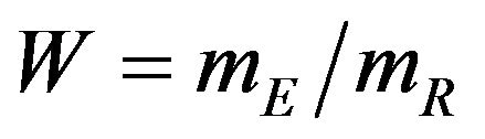 . As under
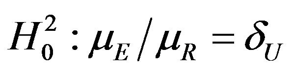 , we set
 . (6.1)
That is, we need to find a cutoff point  that satisfies the equation
 (6.2)
(6.2)
where  is the smallest
  in
in  and
and  . Let
. Let  denote the solution of (6.2) that is less than
 . It follows that
  for all
 .
.
p-Value and Power of the Test
The p-value for the test is
 , (6.3)
where  is the observed ratio. The power function
  at
at , is given by
 (6.4)
(6.4)
Note that the power, for example,  in (6.4) exceeds 0.5 only if
 . For a given
 , it readily follows that
  for all
 . Therefore,
  in (6.4) may be called the minimum power. The test is unbiased.
7. Bootstrap Equivalent Confidence Intervals
In one sample case, for randomly right-censored survival model, Efron has considered using bootstrap to estimate the sampling distribution of , where
![]() is the sample size [5]. He has demonstrated that the sampling distribution of
is the sample size [5]. He has demonstrated that the sampling distribution of  can be estimated by the distribution of
 , where
 denotes the bootstrap Kaplan-Meier estimate. See [5,22] for details on the method(s) of bootstrapping. Let
  denote the Efron’s bootstrap estimate of the median. Then Efron has shown that
  has the same distribution under
  as does
  under F [5]. But we know that m is asymptotically normally distributed with mean
  and variance
 . Therefore, it is reasonable to say that the bootstrap median estimate
  is asymptotically normally distributed with mean equal to the sample median
 ![]() and variance equal to
and variance equal to  [14]. We use this result to formulate a confidence interval based method for assessing non-inferiority of
  compared to
 .
.
Let  be the median estimate based on a bootstrap sample
  taken with replacement from
 , and
, and  denote the median estimate based on a bootstrap sample
  taken with replacement from
 . By the above argument, it follows that
  is asymptotically normally distributed with mean
  and variance
 , and
, and  is asymptotically normally distributed with mean
  and variance
 . Note that
  and
and  are independent. Therefore, the ratio
  has the distribution function
 (7.1)
(7.1)
That is, we plug in the sample estimates of  and
and  in
in  of (4.1) to get an asymptotic distribution of the bootstrap ratio
 . Note that the distribution function
  is completely specified.
Equivalence between the two treatments is often tested by the confidence interval approach, which consists of constructing a  percent confidence interval for the parameter of interest and comparing the constructed confidence interval with the pre-specified equivalence range [9]. In this paper, we use the distribution
  in (7.1) to obtain a
  percent confidence interval for the ratio
  for equivalence testing. A
  percent confidence interval for the ratio
  is given by
 . (7.2)
The interval in (7.2) may be obtained in two ways.
One may tabulate  using SAS PROBNORM and locate the confidence limits. Alternatively, one may write down the quadratic equations of the type shown in (5.2) and (6.2) and solve them. See section 8 for illustration. If the constructed confidence interval
  falls within the equivalence limits
 , then the two groups are considered equivalent. In order to demonstrate non-inferiority, this interval should lie entirely on the positive side of non-inferiority margin. That is, if the confidence interval in (7.2) excludes the non-inferiority margin, then non-inferiority is demonstrated.
8. Sample Size Determination
In the current setting, the standard error of sample median is not explicitly expressed in terms of the number of events. Therefore, we assume exponential model for sample size calculation. That is, we assume that  and
and
 have exponential distribution with means
  and
and
 , respectively. Let
  and
and  represent the maximum likelihood estimates of
  and
and , respectively The median time estimates are given by
and  [13]. Suppose that
  and
and  are the numbers of observed event-times. For simplicity, we assume that
 . The standard errors of
  and
and  are given by
and , respectively. We describe the sample size determination for the test for the upper inequality. That is, we consider testing
8.1. Power Approach
We assume that  is given. That is,
  is known. To be consistent with
 , we set
 . Therefore, we have
 . The null distribution of W is given by
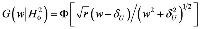 (8.1)
(8.1)
We note that the distribution function  in (8.1) is a function of
  and it does not explicitly depend on
  or
or . We find the cut-off point
  for a level
 ![]() test either by solving
test either by solving 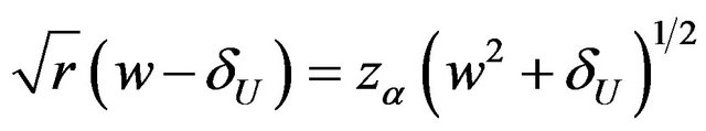 or by tabulating
  in (8.1). The power
  at
at , as a function of
 , is given by
 (8.2)
(8.2)
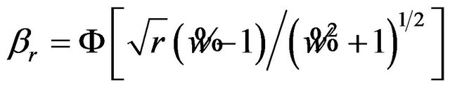
We calculate the optimal number of events  per arm, which yields a power of 0.8 for a test of size 0.05 by iteration. We start with
 . Find
 , where
 . Next, we calculate the power
  given in (8.2). If the power is less than 0.8, we increase
 , and repeat the procedure. We note that when the non-inferiority margin
 , the required number of events per arm is
 . Similarly, for
 , the number of events required per arm is
 . For testing
  versus
 , one needs
  events per arm to achieve a power of 0.8 at
 .
.
8.2. Bootstrap Confidence Interval Approach
In this setting, the distribution function of  is
is
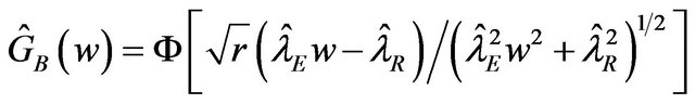 .
.
To find an optimal sample size, we use  to find a
  percent confidence interval. We set
and solve for
The roots of this quadratic equation are given by
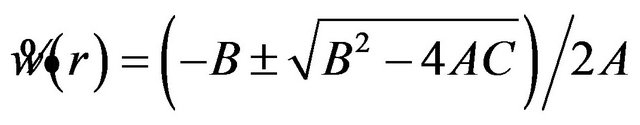 , where
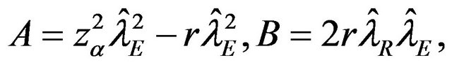 and
and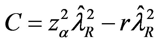 .
.
Let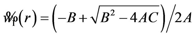 , and
, and
 .
.
Note that  for
for . Then the interval
  is a
is a  confidence interval. The endpoints of the desired confidence interval are expressed in terms of
 . Next, we propose to find
 , an optimal r satisfying
  where d is a pre-specified constant. Ideally, the choice of d should depend on the width of
  or
or . Note that the difference
  is written as
 . A closed form expression for
is not available. We note that  for
for . The optimal number of events per arm
  is the smallest
 such that
 . The value of
  is found by a simple computer search. We have provided values of
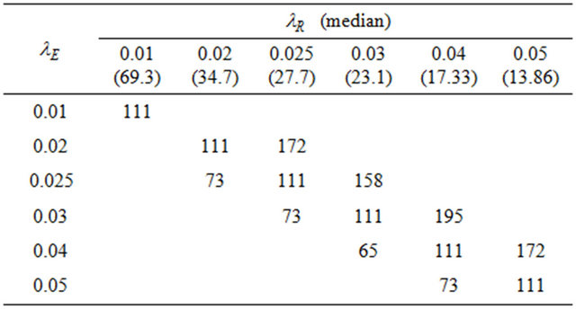
  in Tables 1 and 2 below when
  and
and , respectively. In doing so, we have selected the pairs
  for which non-inferiority (or equivalence) investigation makes sense.
9. Stratified Analysis
In most phase 3 studies, stratified randomization is adopted. That is, subjects are grouped according to covariate values such as age group and baseline performance status prior to randomization and subjects are then randomized within strata.
Within each stratum, a separate randomization sequence to allocate subjects to treatment groups is used. In this section, we extend the above test procedure to clinical trials, which consist of  strata. Consequently, it is necessary to add a second subscript,
  , everywhere, except that
  is assumed constant for all
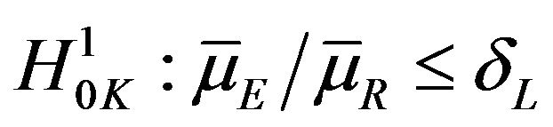
 . We now consider testing the null hypothesis
  for all
  against the alternative hypothesis
  for all
 , and
, and  for some
 . If we choose the simple null hypothesis
 to be the one containing the equality statement, we have
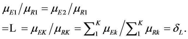
That is, it is possible to restate the null and alternative hypotheses in terms of the sums of strata medians. Let
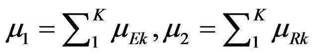 . Then our objective is to test
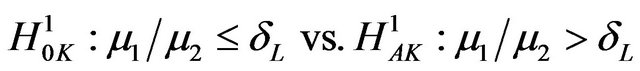 (9.1)
(9.1)
Consequently, we set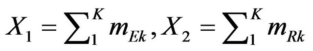 ,
,  and
and . Now
. Now  is normally distributed with mean
  and variance
  and
and  is
is
Table 1. Optimal numbers of events r* per arm for α = 0.025 and d = 0.45.
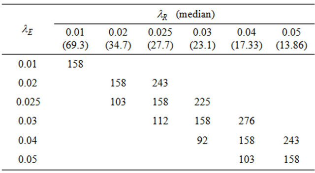
Table 2. Optimal numbers of events r* per arm for α = 0.05 and d = 0.45.
normally distributed with mean  and variance
 . Now let
 . The ratio W follows the F-H distribution. The null distribution function of W is given by
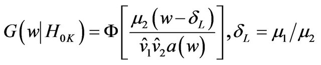 , and
, and
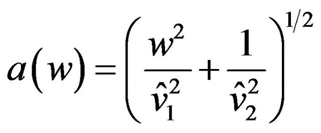 , (9.2)
where  and
and  are estimates of
  and
and , respectively. Reject
  in favor of
 if
if  where
where
 . The cut-off point
  satisfies the equation
 . Note that
 .
.
Let , where
  is a rectangle defined by the
  percent confidence intervals on
  and
and . As earlier, let
  represent the smallest
  in
in  and
and . This results in
 . Therefore, the rule that rejects
  in favor of
  for
for  is a level
 ![]() test.
test.
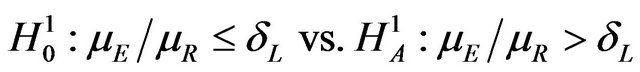
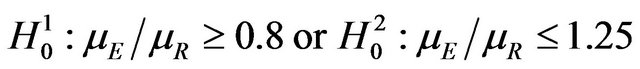
10. Test for Equivalence
The objective is to test
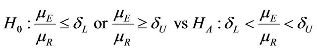 , (10.1)
where the interval  is called equivalence range in clinical trials terminology. The equivalence range may be of the form
  for some
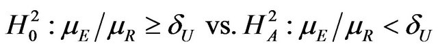
 . We use the well-known two one-sided tests (TOST) approach to test the null hypothesis
  against the alternative hypothesis
  given in (10.1). We first test the following two one-sided hypotheses
 vs
vs , and
, and
 vs
vs 
and then combine the results according intersection-union principle. We have already outlined the two onesided tests in Sections 5 and 6 above. The null hypothesis  is rejected in favor of
  at level
![]() , if both hypotheses
, if both hypotheses  and
and  are rejected at level
![]() . As indicated by Berger and Hsu [9], this test can be quite conservative. We define the p-value as the
. As indicated by Berger and Hsu [9], this test can be quite conservative. We define the p-value as the , where
  and
and  are defined in (5.5) and (6.3), respectively.
Next, we discuss the power of the test of  versus
  of (10.1). We evaluate the power of the test at the alternative
 . Note that we reject
  if
if  and we reject
  if
if , where
  and
and  are determined as explained in Sections 5 and 6, respectively. Intuitively, the power of the test is
For , the power
  is
is
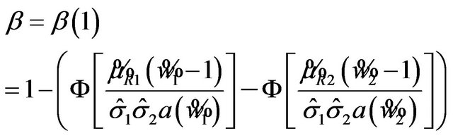 . (10.2)
However, this power may be low in some cases. Then one may use Table 1 or Table 2 for sample size determination.
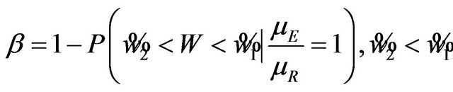
In Figure 2 we have provided a graphical summarization of testing for equivalence at .
.
Figure 2 contains the density functions of  for noninferiority margin
 . Here we have used
 , and
, and  in all three cases. Note that
  and
and  are the cutoff points and the area marked by (1) and (2) represent the level of significance
 ![]() for testing
for testing  and
and , respectively. The total area represented by (1) + (2) + (3) + (4) is the power of the equivalence test given in (10.2).
11. Concluding Remarks
We deal with the ratio  directly, and therefore,
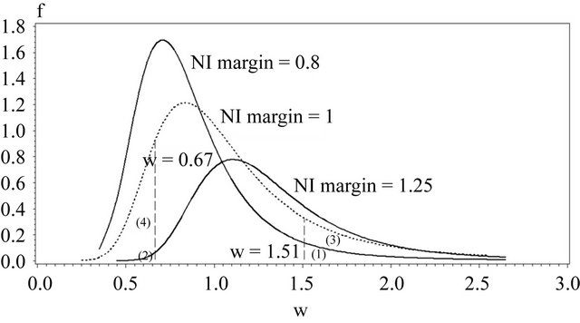
Figure 2. Overview of the equivalence test.
our approach is easy for clinicians to understand. Existing test procedures for assessing non-inferiority and equivalence require hazard rates under the two treatment arms to be proportional. Our test proposed in this paper is free of this requirement and therefore, has wider applicability.
The power definitions in (5.6) and (6.4) may be considered as alternative to the power definitions in [20,21].
It may be recalled here that the Mantel-Haenszel test [23] is often called an average partial association statistic. Here we have a parallel situation. Note that the null hypothesis  in (9.1) may be written as
 , where
 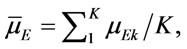 and
and
 . Therefore, the procedure in Section 9 tests the null hypothesis on the ratio of averages of strata medians.
12. Acknowledgements
This article reflects the views of the author and should not be construed to represent FDA’s views or policies. No official support or endorsement of this article by the Food and Drug Administration is intended or should be inferred.
REFERENCES
- “E-10: Guidance on Choice of Control Group in Clinical Trials,” International Conference on Harmonization of Technical Requirements for Registration of Pharmaceuticals for Human Use (ICH), Vol. 64, No. 185, 2000, pp. 51767-51780.
- R. B. D’Agostino, J. M. Massaro and L. M. Sullivan, “Non-Inferiority Trials: Design Concepts and Issues— The Encounters of Academic Consultants in Statistics,” Statistics in Medicine, Vol. 22, No. 2, 2003, pp. 169-186. doi:10.1002/sim.1425
- G. G. Koch, “Non-Inferiority in Confirmatory Active Control Clinical Trials: Concepts and Statistical Methods,” American Statistical Association: FDA/Industry Workshop, Washington, D.C., 2004.
- S. Wellek, “Testing Statistical Hypothesis of Equivalence,” CHAPMAN & HALL/CRC, New York, 2003.
- B. Efron, “Censored Data and the Bootstrap,” Journal of the American Statistical Association, Vol. 76, No. 374, 1981, pp. 312-319. doi:10.1080/01621459.1981.10477650
- R. Simon, “Confidence Intervals for Reporting Results of Clinical Trials,” Annals of Internal Medicine, Vol. 105, No. 3, 1986, pp. 429-435.
- L. Rubinstein, M. Gail and T. Santner, “Planning the Duration of a Comparative Clinical Trial with Loss to Follow-Up and a Period of Continued Observation,” Journal of Chronic Disease, Vol. 34, No. 9-10, 1981, pp. 469-479. doi:10.1016/0021-9681(81)90007-2
- D. R. Bristol, “Planning Survival Studies to Compare a Treatment to an Active Control,” Journal of Biopharmaceutical Statistics, Vol. 3, No. 2, 1993, pp. 153-158. doi:10.1080/10543409308835056
- R. L. Berger and J. C. Hsu, “Bioequivalence Trials, Intersection-Union Tests and Equivalence Confidence Sets,” Statistical Science, Vol. 11, No. 4, 1996, pp. 283-319. doi:10.1214/ss/1032280304
- D. Hauschke and L. A. Hothorn, “Letter to the Editor,” Statistics in Medicine, Vol. 26, No. 1, 2007, pp. 230-236. doi:10.1002/sim.2665
- SAS Institute Inc., “SAS/STAT User’s Guide,” Version 8, Cary, 2000.
- R. Brookmeyer and J. Crowley, “A Confidence Interval for the Median Survival Time,” Biometrics, Vol. 38, No. 1, 1982, pp. 29-41. doi:10.2307/2530286
- D. Collett, “Modeling Survival Data in Medical Research,” 1st Edition, Chapman & Hall, London, 1994.
- N. Reid, “Estimating the Median Survival Time,” Biometrika, Vol. 68, No. 3, 1981, pp. 601-608. doi:10.1093/biomet/68.3.601
- G. J. Babu, “A Note on Bootstrapping the Variance of Sample Quantiles,” Annals of the Institute of Statistical Mathematics, Vol. 38, 1985, pp. 439-443. doi:10.1007/BF02482530
- The University of Texas at Austin, “Setting and Resampling in SAS,” 1996. http://ftp.sas.com/techsup/download/stat/jackboot.htm/
- K. M. Keaney and L. J. Wei, “Interim Analyses Based on Median Survival Times,” Biometrika, Vol. 81, No. 2, 1994, pp. 279-286. doi:10.1093/biomet/81.2.279
- E. C. Fieller, “The Distribution of the Index in a Normal Bivariate Population,” Biometrika, Vol. 24, No. 3-4, 1932, pp. 428-440. doi:10.1093/biomet/24.3-4.428
- D. V. Hinkley, “On the Ratio of Two Correlated Normal Variables,” Biometrika, Vol. 56, No. 3, 1969, pp. 635- 639. doi:10.1093/biomet/56.3.635
- K. M. Koti, “Use of the Fieller-Hinkley Distribution of the Ratio of Random Variables in Testing for Non-Inferiority and Equivalence,” Journal of Biopharmaceutical Statistics, Vol. 17, No. 2, 2007, pp. 215-228. doi:10.1080/10543400601177335
- K. M. Koti, “New Tests for Null Hypothesis of NonUnity Ratio of Proportions,” Journal of Biopharmaceutical Statistics, Vol. 17, No. 2, 2007, pp. 229-245. doi:10.1080/10543400601177426
- B. Efron and R. J. Tibshirani, “An Introduction to the Bootstrap,” Chapman & Hall, New York, 1993.
- M. E. Stokes, C. S. Davis and G. G. Koch, “Categorical Data Analysis Using the SAS System,” SAS Institute Inc., Cary, 1995.