Open Journal of Statistics
Vol.2 No.5(2012), Article ID:25362,5 pages DOI:10.4236/ojs.2012.25059
Bootstrap-T Technique for Minimax Multivariate Control Chart
1Distance Learning Institute, University of Lagos, Lagos, Nigeria
2Department of Mathematical Sciences, Redeemer’s University, Redemption City, Nigeria
Email: samadek_2017@yahoo.co.uk
Received August 8, 2012; revised September 10, 2012; accepted September 22, 2012
Keywords: Bootstrap; Minimax; Multivariate Data; Control Limits; Process Control
ABSTRACT
Bootstrap methods are considered in the application of statistical process control because they can deal with unknown distributions and are easy to calculate using a personal computer. In this study we propose the use of bootstrap-t multivariate control technique on the minimax control chart. The technique takes care of correlated variables as well as the requirement of the distributional assumptions needed for the operation of the minimax control chart. The bootstrap-t technique provides the mean  of all the bootstrap estimators
  where
where ![]() is the estimate using the
is the estimate using the  bootstrap sample and B is the number of bootstraps. The computation of the proposed bootstrap-t minimax statistic was performed on the values obtained from the bootstrap estimation. This method was used to determine the position of the four control limits of the minimax control chart. The bootstrap-t approach introduced to minimax multivariate control chart helps to detect shifts in the mean vector of a multivariate process and it overcomes the computational complexity of obtaining the distribution of multivariate data.
1. Introduction
The high rate of interest in multivariate control charts is now on increase after a volume of research in all areas of univariate control charts. Multivariate control charts have the advantage of being able to monitor multiple quality characteristics simultaneously for both changes in the mean vector and the correlation structure while maintaining a specified probability of Type I error (α). Multivariate control charts are at a disadvantage because it is difficult to identify which subset of the quality characteristics are responsible for a signal since any single characteristic or combination of characteristics could have experienced a shift in mean value, variance, or correlation.
Many industrial applications today have several correlated quality characteristics that needed to be monitored simultaneously. Each item in the sample is inspected and the values of each of its quality characteristics are determined. The information from the sample, contained in the sample statistics, is used to determine whether the process appears to be in control with reasonable variation. If the mean vector of one or more of the variables appears to have deviated from its desired value, or if the variation in one or more of the variables seems to have increased, the process is considered out of control [1].
The development of multivariate control charts originates from the work by [2]. [3] provided a general framework on constructing control charts for both univariate and multivariate situations. [4] proposed a bootstrap control chart that can monitor both independent and dependent observations. [5] discussed the performance of techniques for constructing bootstrap control charts, [6] proposed a bootstrap control chart based on the BirnbaumSaunders distribution, and [7] proposed median control charts whose control limits were determined by estimating the variance of the sample median via the bootstrap technique. Recent work by [8] proposed a bootstrapbased multivariate T2 control chart that can efficiently monitor a process when the distribution of observed data is non-normal or unknown. The concept of minimax control chart for multivariate quality control was introduced by [9]. The minimax control chart uses the joint probability distribution of the maximum and minimum standardized sample means to obtain the control limits for monitoring purposes. This chart operates under the assumptions of normality and uncorrelated variable. [10] uses a non-linear polynomial function approach to solve the problem of normality assumption needed to obtain the control limits for the minimax control chart. In this paper, we introduce the concept of bootstrapping technique to address the issues of uncorrelated variables as well as the distributional assumptions of minimax control charts. Furthermore, the control limits for minimax control chart were determined for varying level of significance to enable process control operators to make a robust choice of control limits that will suite their purpose.
2. Method
The minimax control chart developed by [9] is similar to the charts proposed by [11] and [12]. The minimax control chart also uses the minimum and maximum standardized sample means to make the decision if the process should be considered in control or out of control. However, the minimax chart uses both lower and upper control limits on both the maximum and minimum standardized sample means. This is facilitated by the development of the capability to determine the value of the joint density function of the maximum and minimum standardized sample means. This not only facilitates a method for setting the control limits, but also allows for the comparison of the performance of the minimax chart relative to other charts through computation of the outof-control average run length.
The minimax chart operates by controlling the minimum and maximum standardized sample means. The correlation between the quality characteristic variables, which is assumed to be known, is incorporated into the construction of the control limits for the minimum and maximum standardized sample mean. In addition, the chart operates at a relatively low and fixed probability of Type I error (α). There are several advantages of using the minimax control chart. Although the construction of the chart is fairly complex, the application of the chart is extremely straight-forward. The computations involve the standardization of each of the mean quality characteristic values. The maximum and minimum of these values are then plotted, each against its upper and lower control limits.
The minimax chart monitors p quality characteristics simultaneously. At fixed time intervals, a sample of size n is taken and the value of each of the quality characteristics is determined. Let Xij represent the value of quality characteristic i of item j for  and
and , and let
 ![]() contains the sample mean value for each quality characteristic. Although the observations may be correlated within each sample, the samples are assumed independent of each other. In addition, it is assumed that
contains the sample mean value for each quality characteristic. Although the observations may be correlated within each sample, the samples are assumed independent of each other. In addition, it is assumed that  is distributed with a multivariate normal distribution with known process mean vector
  and covariance matrix
 , where
  is the variance of the ith quality characteristic and
  is the covariance between the ith quality characteristic and the jth quality characteristic. The covariance structure is assumed to remain stable over time leaving only a shift in the mean vector to cause an out-of-control situation.
The minimax chart requires the minimum and maximum standardized sample means to fall between their respective control limits. In order to obtain the minimum standardized sample mean  and the maximum standardized sample mean
 , each of the elements of the sample mean vector,
  is standardize using
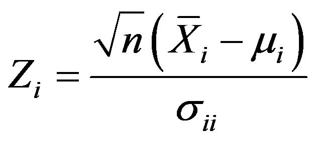 (1)
(1)
Note that Zi is simply the standardized sample mean for the ith quality measure and Z[i] is an order statistic defining the ith smallest value of the p standardized sample means. Therefore Z[1] and Z[p] are determined from  There are four control limits for the minimax chart. These are UCL[1] and LCL[1] i.e. the respective upper and lower control limits for Z[1] and UCL[p] and LCL[p] are the respective upper and lower control limits for Z[p]. It should be noted that the minimax chart is essentially two dependent charts. One chart monitors and controls Z[1] and the other chart monitors and controls Z[p]. The charts are dependent because the joint distribution of Z[1] and Z[p] is used to construct the control limits. The probability of a Type I error, α, is the sum of the probabilities of a Type I error in the Z[1] chart,
  , and a Type I error in the Z[p] chart, α[p].
In this paper, the control limits proposed by [9] for the minimax control chart were adopted. These control limits are given in Equation (2)
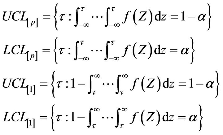 (2)
(2)
These control limits are function of the probability of Type I error ,
, ![]() and the distribution of the transformed variable. It is worthy to note that the control limits depends heavily on the value of
and the distribution of the transformed variable. It is worthy to note that the control limits depends heavily on the value of ![]() chosen. Therefore, we consider varying the value of
chosen. Therefore, we consider varying the value of ![]() to obtain the four control limits of the minimax control chart.
to obtain the four control limits of the minimax control chart.
Bootstrap-T Method
The bootstrap method, introduced by [13], is a powerful tool for estimating the sampling distribution of a given statistic. The bootstrap estimate of the sampling distribution is generally better than the normal approximation based on the central limit theorem (cf. [14] and [15]), even if the statistic is not standardized (cf. [16] and [17]). Let  be an iid sample following the distribution F with mean,
  and variance
 . The standard bootstrap procedure is to draw with replacement a random sample of size N from
 . Denote the bootstrap sample by
  and denote their mean and standard deviation by
  and
and . Suppose FN indicate the empirical distribution of
 then the sampling distribution of
  under FN
is the bootstrap approximation of the sampling distribution of  under F. Its approximation error is shown to be negligible by the proposition derived by [14] and [15]). The bootstrap technique provides the mean
  of all the bootstrap estimators
 (3)
(3)
where ![]() is the estimate using the
is the estimate using the  bootstrap sample and B is the number of bootstraps.
The bootstrap handles cases where a standard distribution cannot be assumed. The control limit is estimated by resampling the observed data to estimate the distribution of the observed variable. For many problems in statistics, we are interested in the distribution of values from a random sample of the population. If the underlying distribution from which the values are drawn is known, we can use developed theory to generate the sampling distribution. [13] proposed the use of bootstrapping when there is little or no significant information about the underlying distribution. The idea behind the bootstrap is very simple, namely that (in the absence of any other information), the sample itself offers the best guide of the sampling distribution. By resampling with replacement from the original sample, we can create a bootstrap sample, and use the empirical distribution of our estimator in a large number of such bootstrapped samples to construct confidence intervals and tests for significance. In this paper, the bootstrap-t method is employed.
The bootstrap-t method procedure directly estimates the standard normal distribution (Z) from the data, much like the use of the normal and t tables. We generate B bootstrap samples  and for each we compute
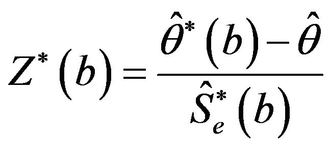 (4)
(4)
where  is the value of
  for the bootstrap sample
 , and
, and  is the estimated standard error of
  for the bootstrap sample
 . The
. The  percentile of
  is estimated by the value
  such that
 (5)
(5)
where ![]() is the B·
is the B· value in the ordered list of the smallest value of the
  in interval
 . For instance, if
 , the estimate of the 90% point is the
  smallest value of the
 . The “bootstrap-t” confidence interval is
In this study we adopt the bootstrap-t method given in Equation (4) to generate the data set that we used to obtain the control limits for the minimax control chart developed by [9]. The vector ,
,  is now defined as the standardized bootstrap sample mean vector. The maximum sample mean
  is defined as the maximum of the elements of the vector
 that is,
![]() . Also, the minimum standardized sample mean
. Also, the minimum standardized sample mean  is defined as the minimum of the elements of the bootstrap vector
 as given by
![]() . These minimum and maximum statistics are then implemented on the control limits in Equation (2).
. These minimum and maximum statistics are then implemented on the control limits in Equation (2).
3. Results
The data used in this study for illustrative purpose were collected from the production line of a soft drinks manufacturing company in Nigeria. We considered five important quality characteristics of the soft drink. These are: X1 = Contents in ml, X2 = Brix, X3 = pressure, X4 = CO2, and X5 = Temperature. The data was first tested for autocorrelation and it was discovered that the data are uncorrelated. Thereafter, the data was bootstrapped using the approach described in Section 2. The result of the bootstrap analysis is presented in Table 1.
To obtain the control limits in Equation (2), an algorithm was developed and implemented on C language using different levels of significance (![]() ) from 1% to 50%. The Control limits for five variables case considered in this study were determined for varying level of significance from 0.01 to 0.5. The obtained control limits are presented in Table 2
) from 1% to 50%. The Control limits for five variables case considered in this study were determined for varying level of significance from 0.01 to 0.5. The obtained control limits are presented in Table 2
4. Discussion of Results
The results in Table 1 represent the summary of the descriptive statistics of the bootstrap data and the original data from the production line, where , SD*(b), and Z*(b) are the mean, standard deviation, and the standardized values of the bootstrapped data. The bootstrap statistics shows the same feature with the real data. The Control limits in Table 2 are obtained for five vari-
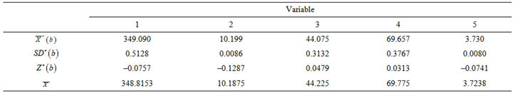
Table 1. Summary of result for the bootstrap data for five variables.
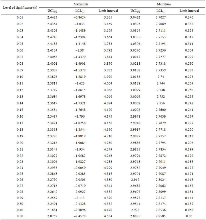
Table 2. The minimax control limits for varying level of significance (α).
ables scenario. It should be noted that the control limits for situation for more than five variables can be obtained by an extension of the program used in this study. From the bootstrap data, the value of the minimum  and the value of the maximum
 . If the management is interested in taking decision based on 1% level of significance
 , then the control limits from Table 2 will be
 ,
,  ,
,  and
and . Therefore,< the maximum value
 will be within the control limits whereas, the minimum value
  will be lying outside the lower control limit. However, if the management is interested in taking decision based on 5% level of significance
 , then the control limits from Table 2 will be
 ,
,  ,
,  and
and . This will give the same conclusion as that of when
  is used. Furthermore, the results show that the control limit interval increases as the level of significance increases. For instance, the control limit interval when
  are 3.304 for the maximum and 0.339 for the minimum. When
 , the control limit intervals are 3.734 for the maximum and 0.311 for the minimum.
5. Conclusion
This work used the bootstrap techniques to set up the control limits for a minimax control chart. The control limits for minimax control chart were determined for varying level of significance to enable process control operators to make a robust choice of control limits that will suite their purpose. Furthermore, the derived control limits for a five variable scnerio showed that the smaller the control limit interval, the higher the false alarm rate and hence high Type I error probability. Therefore, the obtained value of control limits in Table 2 will help the management to take decision on the level of significance to use for monitoring purpose. An extension or review of the used algorithm will provide the control limits for multivariate problem with less or greater than five variables.
REFERENCES
- J. Rehmert, “A Performance Analysis of the Minimax Multivariate Quality Control Chart,” Master of Science Dissertation, Department of Industrial and Systems Engineering, Virginia Polytechnic Institute and State University, Blacksburg, 1997
- H. Hotelling, “Multivariable Quality Control—Illustrated by the Air Testing of Sample Bombsight,” In: C. Eisenhart, M. W. Hastay and W. A. Wallis, Eds., Techniques of Statistical Analysis, McGraw Hill, New York, 1947, pp. 110-122.
- A. M. Polansky, “A General Framework for Constructing Control Charts,” Quality and Reliability Engineering International, Vol. 21, No. 6, 2005, pp. 633-653.
- R. Y. Liu and J. Tang, “Control Charts for Dependent and Independent Measurements Based on the Bootstrap,” Journal of the American Statistical Association, Vol. 91, No. 436, 1996, pp. 1694-1700.
- I. A. Jones and W. H. Woodall, “The Performance of Bootstrap Control Charts,” Journal of Quality Technology, Vol. 30, No. 4, 1998, pp. 362-375.
- Y. L. Lio and C. Park, “A Bootstrap Control Chart for Birnbaum-Saunders Percentiles,” Quality and Reliability Engineering International, Vol. 24, No. 5, 2008, pp. 585- 600.
- H. I. Park, “Median Control Charts Based on Bootstrap Method,” Communications in Statistics—Simulation and Computation, Vol. 38, No. 1, 2009, pp. 558-570.
- P. Phaladiganon, S. B. Kim, V. C. P. Chen, J. G. Baek and S. K. Park, “Bootstrap-Based T2 Multivariate Control Charts,” Communications in Statistics—Simulation and Computation, Vol. 40, No. 5, 2011, pp. 645-662. doi:10.1080/03610918.2010.549989
- A. Sepulveda, “The Minimax Control Chart for Multivariate Quality Control,” Ph.D. Dissertation, Virginia Polytechnic Institute and State University, Department of Industrial and Systems Engineering, Blacksburg, 1996.
- J. A. Adewara, K. S. Adekeye, O. E. Asiribo and S. B. Adejuyigbe, “Minimax Multivariate Control Chart Using a Polynomial Function,” Applied Mathematics, Vol. 2, No. 12, 2011, pp. 1539-1545. doi:4236/am..2011.212219
- A. J. Hayter and K. L. Tsui, “Identification and Quantification in Multivariate Quality Control Problems,” Journal of Quality Technology, Vol. 26, No. 3, 1994, pp. 197-208.
- N. H. Timm, “Multivariate Quality Control Using Finite Intersection Tests,” Journal of Quality Technology, Vol. 28, No. 2, 1996, pp. 233-243.
- B. Efron, “Bootstrap Methods: Another Look at the Jackknife,” The Annals of Statistics, Vol. 7, No. 1, 1979, pp. 1-26. doi:10.1214/aos/1176344552
- P. J. Bickel and D. A. Freedman, “Some Asymptotic Theory for the Bootstrap,” The Annals of Statistics, Vol. 9, No. 6, 1981, pp. 1196-1217.
- K. Singh, “On the Asymptotic Accuracy of Efron’s Bootstrap,” The Annals of Statistics, Vol. 9, No. 6, 1981, pp. 1187-1195.
- R. J. Beran, “Estimated Sampling Distributions: The Bootstrap and Competitors,” The Annals of Statistics, Vol. 10, No. 1, 1982, pp. 212-215.
- R. Liu and K. Singh, “On a Partial Correction by the Bootstrap,” The Annals of Statistics, Vol. 15, No. 4, 1987, pp. 1713-1718.