Open Journal of Microphysics
Vol.3 No.3(2013), Article ID:35702,7 pages DOI:10.4236/ojm.2013.33010
Matrix Quasi-Exactly Solvable Jacobi Elliptic Hamiltonian
Institut de Pédagogie Appliquée, Université du Burundi, Bujumbura, Burundi
Email: nininaha@yahoo.fr
Copyright © 2013 Ancilla Nininahazwe. This is an open access article distributed under the Creative Commons Attribution License, which permits unrestricted use, distribution, and reproduction in any medium, provided the original work is properly cited.
Received April 11, 2013; revised May 12, 2013; accepted May 20, 2013
Keywords: Technology; Preference for Quality; Volume of Trade; Vertical Intra-Industry Trade
ABSTRACT
We construct a new example of 2 × 2-matrix quasi-exactly solvable (QES) Hamiltonian which is associated to a potential depending on the Jacobi elliptic functions. We establish three necessary and sufficient algebraic conditions for the previous operator to have an invariant vector space whose generic elements are polynomials. This operator is called quasi-exactly solvable.
1. Introduction
In quantum physics, one of the main mathematical problems consists in constructing the spectrum of a linear operator defined on a suitable domain of Hilbert space. In most cases, this type of problem cannot be explicitly solved, in other words the eigenvalues of the Hamiltonian cannot be computed algebraically. However, in few cases, some of which turn out to be physically fundamental, the spectrum can indeed be found explicitly. The two major examples of this kind are the celebrated harmonic quantum oscillator and the hydrogen atom (i.e. 3- dimensional Schrödinger equation coupled to an external Coulomb potential). These examples are called exactly solvable in the sense that the full spectrum of the Hamiltonian is found explicitly.
In the last few years, a new class of operators which is intermediate to exactly solvable and non solvable operators has been discovered [1-4]: the quasi-exactly solvable (QES) operators, for which a finite part of the spectrum can computed algebraically.
Although scalar QES operators have been classified in one variable [5] and in several variables [6], a classification of matrix QES operators is still missing.
More recently, interesting tools for classification of 2 × 2-matrix QES operators in one spatial dimensional [7- 9] and in creation and annihilation operators [10] have been constructed.
In the Ref. [9], PT-symmetric, QES 2 × 2-matrix Hamiltonians are analyzed with the emphasis set on the reality properties of the eigenvalues. The authors considered both trigonometric and hyperbolic 2 × 2-matrix Hamiltonians.
A set of necessary and sufficient conditions (i.e. QES conditions) for 2 × 2-matrix operators to preserve a vector space of polynomials have been proposed. These QES conditions constitute the so-called QES analytic method.
This paper is organized as follows: In the Section 2, based on the Ref. [9], we briefly recall the QES analytic method used to investigate the quasi-exact solvability of 2 × 2-matrix operators. In Section 3, along the same lines as in the Ref. [9], we apply the QES analytic method in order to construct a new 2 × 2-matrix QES Hamiltonian depending on Jacobi elliptic functions. We will consider two values of the constant δ: the case δ = 1 and the case δ = 2. The interesting results will be found.
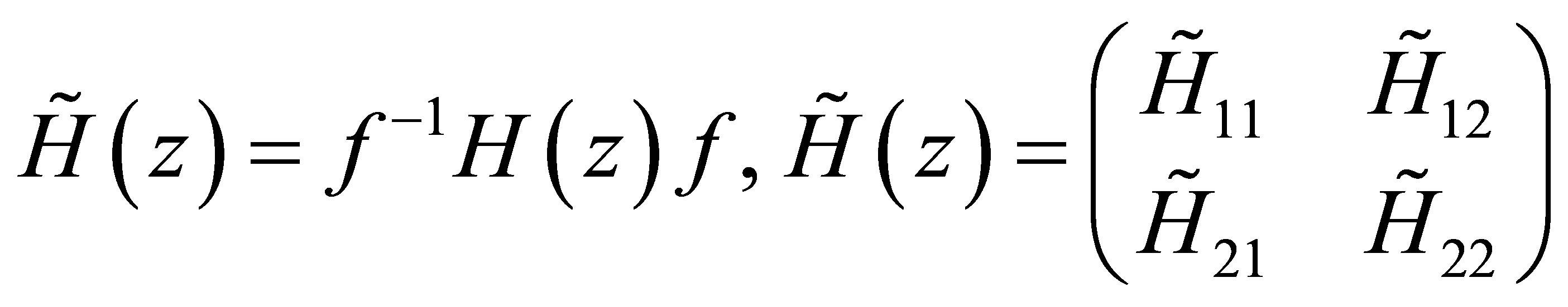
2. QES Analytic Method
A general test to check whether a  -matrix differential operator H (in a variable
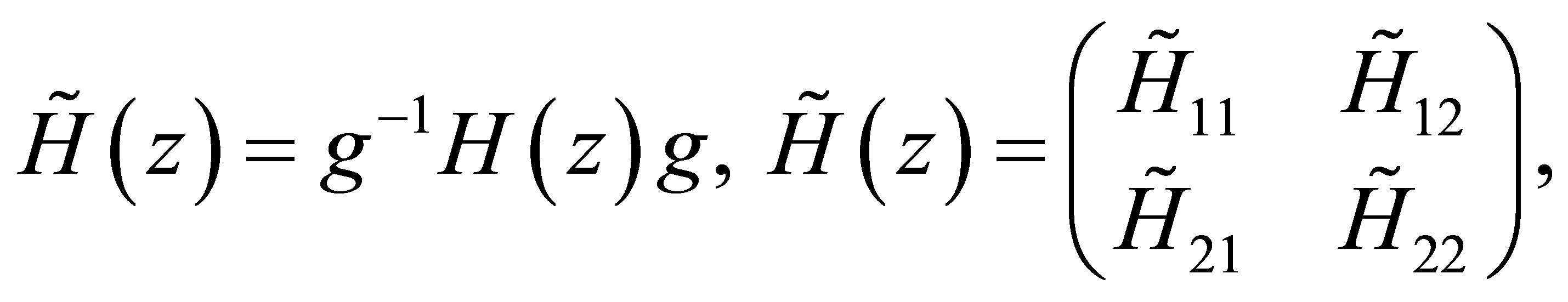
![]() ) preserves a vector space whose components are polynomials is proposed [9]. After a gauge transformation and a change of variable on the operator H lead to a new operator
) preserves a vector space whose components are polynomials is proposed [9]. After a gauge transformation and a change of variable on the operator H lead to a new operator  which can be decomposed as follows
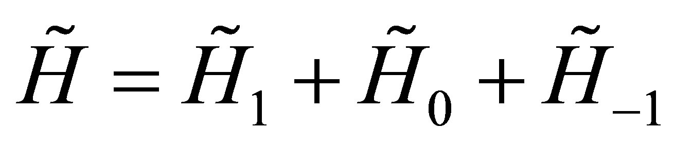 , (1)
, (1)
with
 .
.
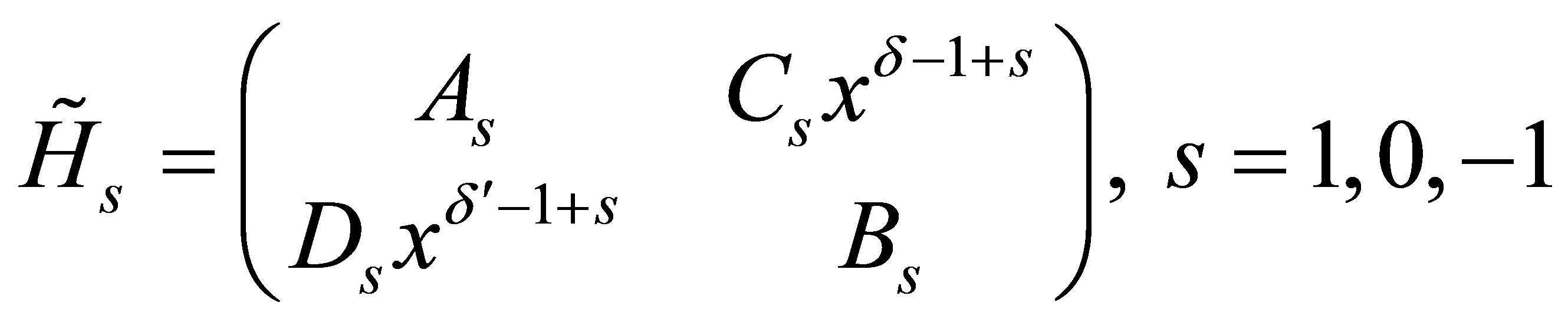
Here 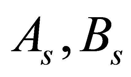 denote homogeneous differential operators, Cs, Ds are arbitrary constant and
  are integers. More precisely, the diagonal components of
  are differential operators and the off-diagonal components
![]() and
and ![]() are respectively proportional to
are respectively proportional to  and
and  with
with  and
and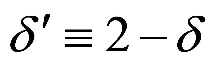 . The operators
  and
and  have lower degrees in all their components than the corresponding components in
 .
.
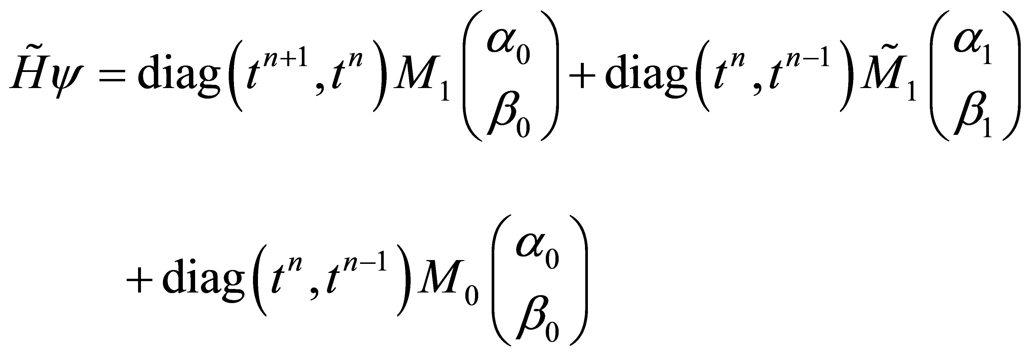
In order to obtain QES conditions for , the generic vector of the vector space
  is
is
 , (2)
, (2)
Where 
 are complex parameters. As a consequence the 2 × 2-matrices
  are defined by
 (3)
(3)
The three QES conditions for  to have an invariant vector space are as follows [9]
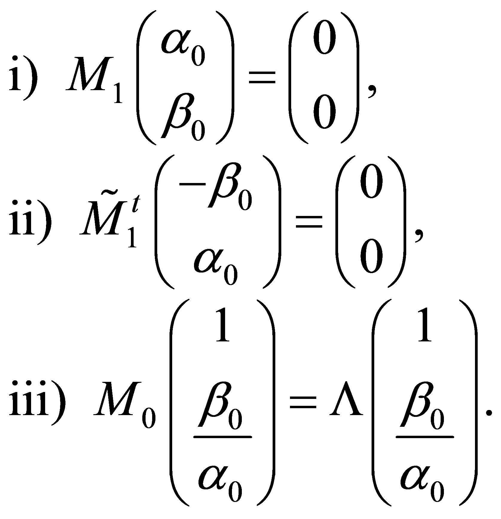 (4)
(4)
In the next step, we will apply in a systematic way the previous QES analytic method in order to construct a 2 × 2-matrix QES Hamiltonian associated to a potential depending on the Jacobi elliptic functions [11,12].
3. QES Jacobi Hamiltonian
3.1. Case δ = 1
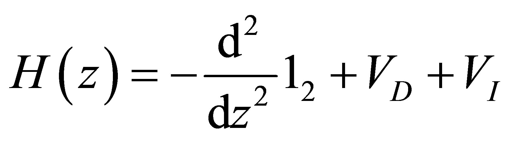
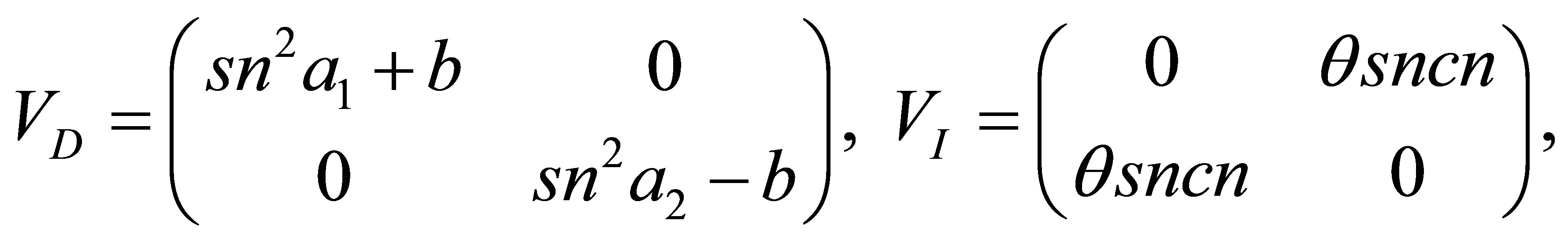
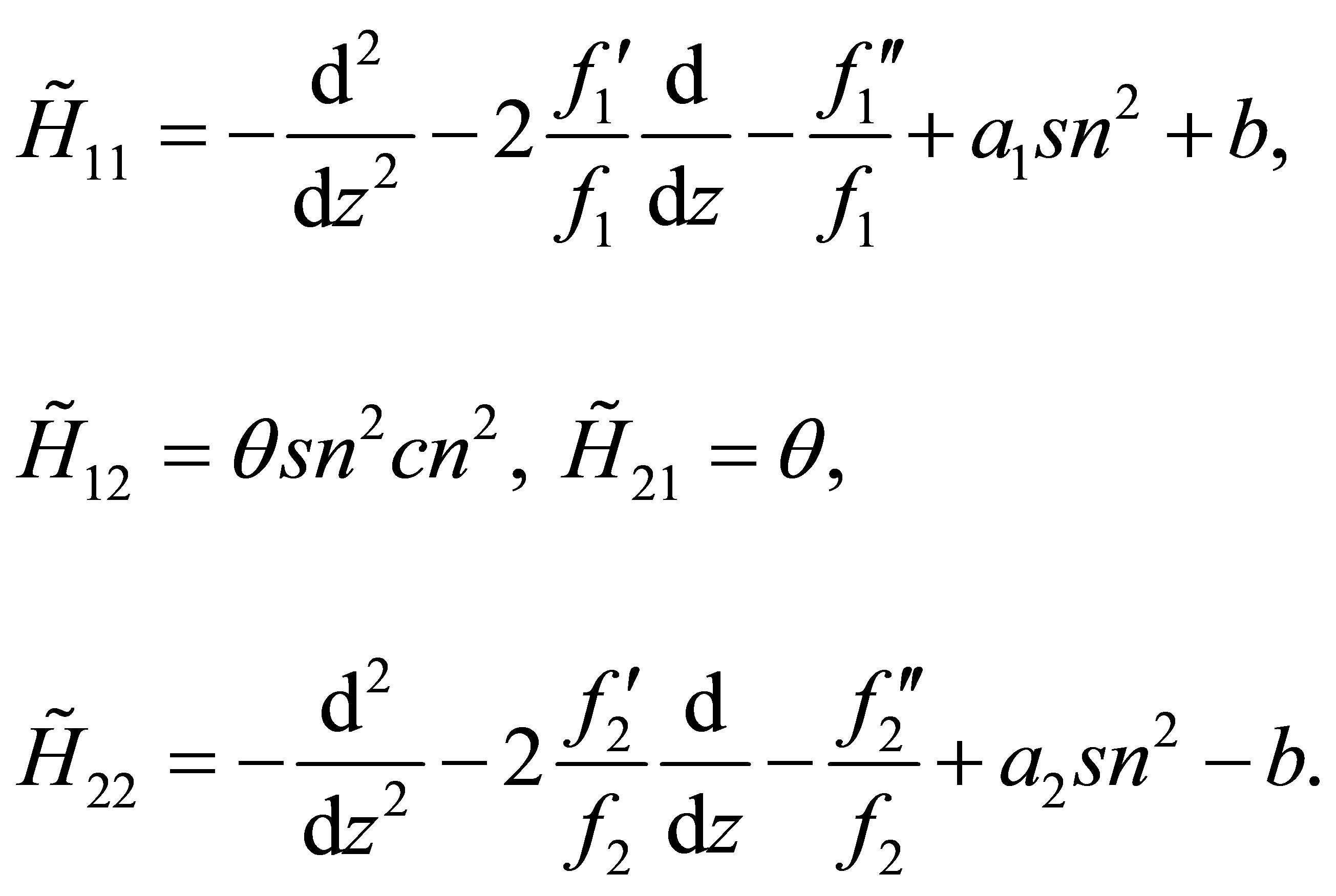
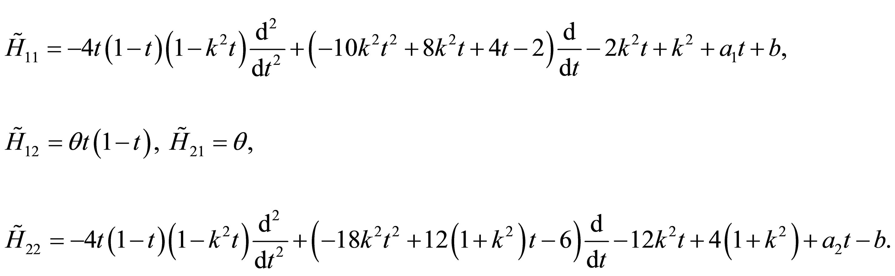
In this section we apply the QES analytic method established previously to check whether a particular 2 × 2-matrix operator is QES. We consider Schrödinger N × N-matrix operator with potential depending on the Jacobi elliptic functions of the form [11]:
 (5)
(5)
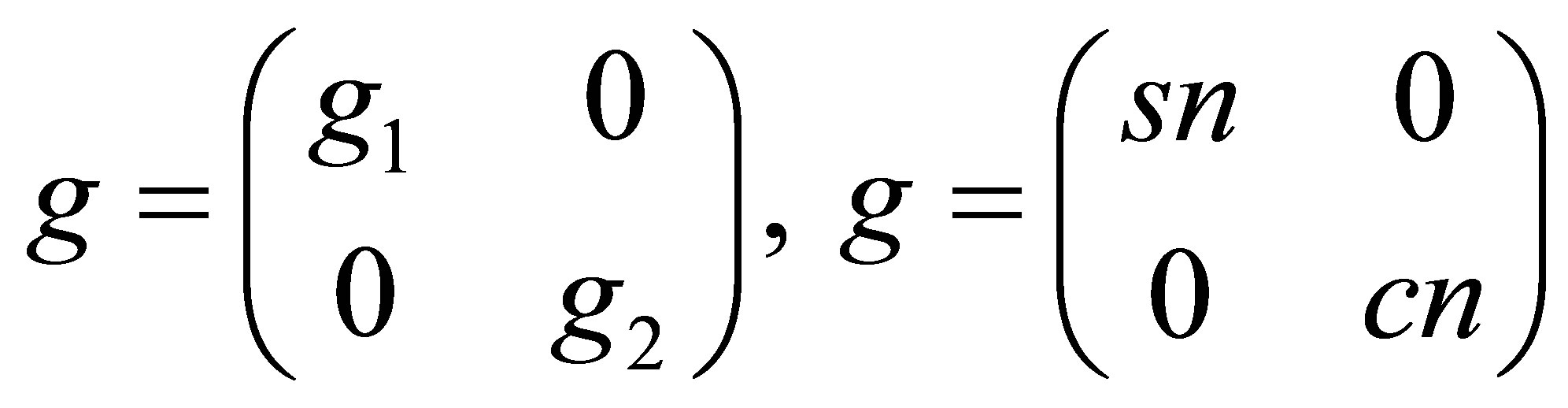
with
 (6)
(6)
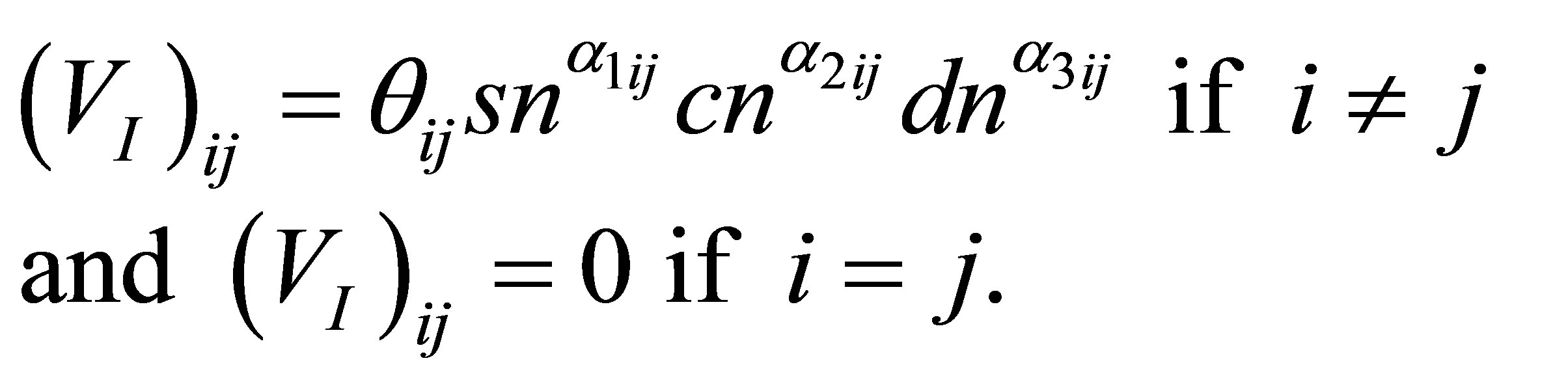
where aj, bj denote real constants (without loss of generality we assume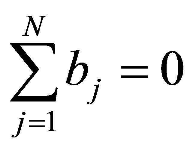 ) and VI is symmetric off-diagonal matrix of the form
Note that the above Hamiltonian is to be considered on the Hilbert space of periodic functions on [0, 4 K(k)].
The properties of the Jacobi functions that are useful to make calculations are listed in the relations (12) and (13).
The case 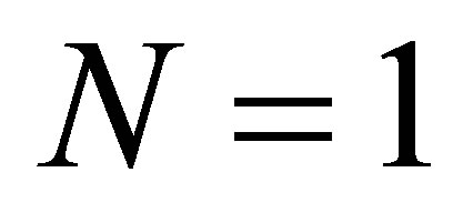 corresponds to the Lamé equation [11]. We will treat in details the case
  which corresponds to the following operator
 (7)
(7)
with
![]() is the matrix identity and
is the matrix identity and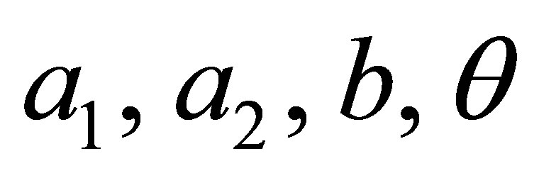
 denote real constants. Note that the sum
  is the potential associated to the Hamiltonian H(z).
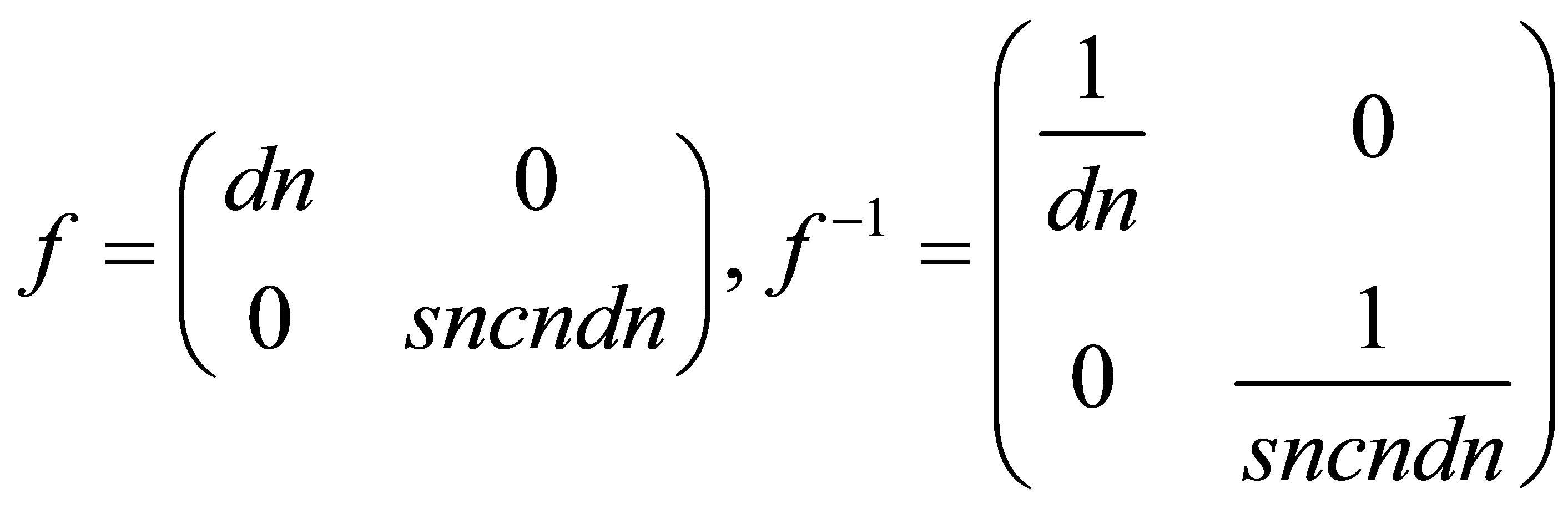
Using the following change of function (i.e. the gauge transformation), the gauge Hamiltonian is written as follows
 (8)
(8)
where
 (9)
(9)
and
 , (10)
Notice that two operators H and  are called equivalent based on the Equation (8).
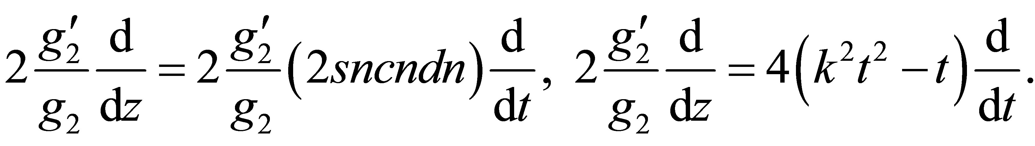
The relevant change of variable consists in posing
 . In particular the differential symbol
is transformed into the following expression
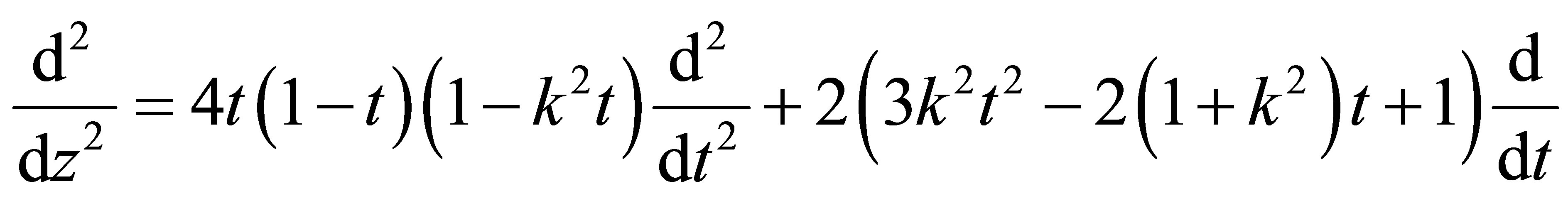 (11)
(11)
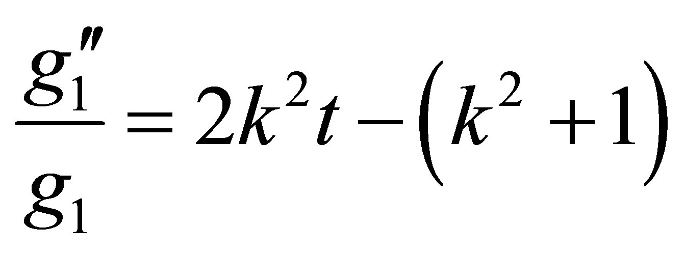
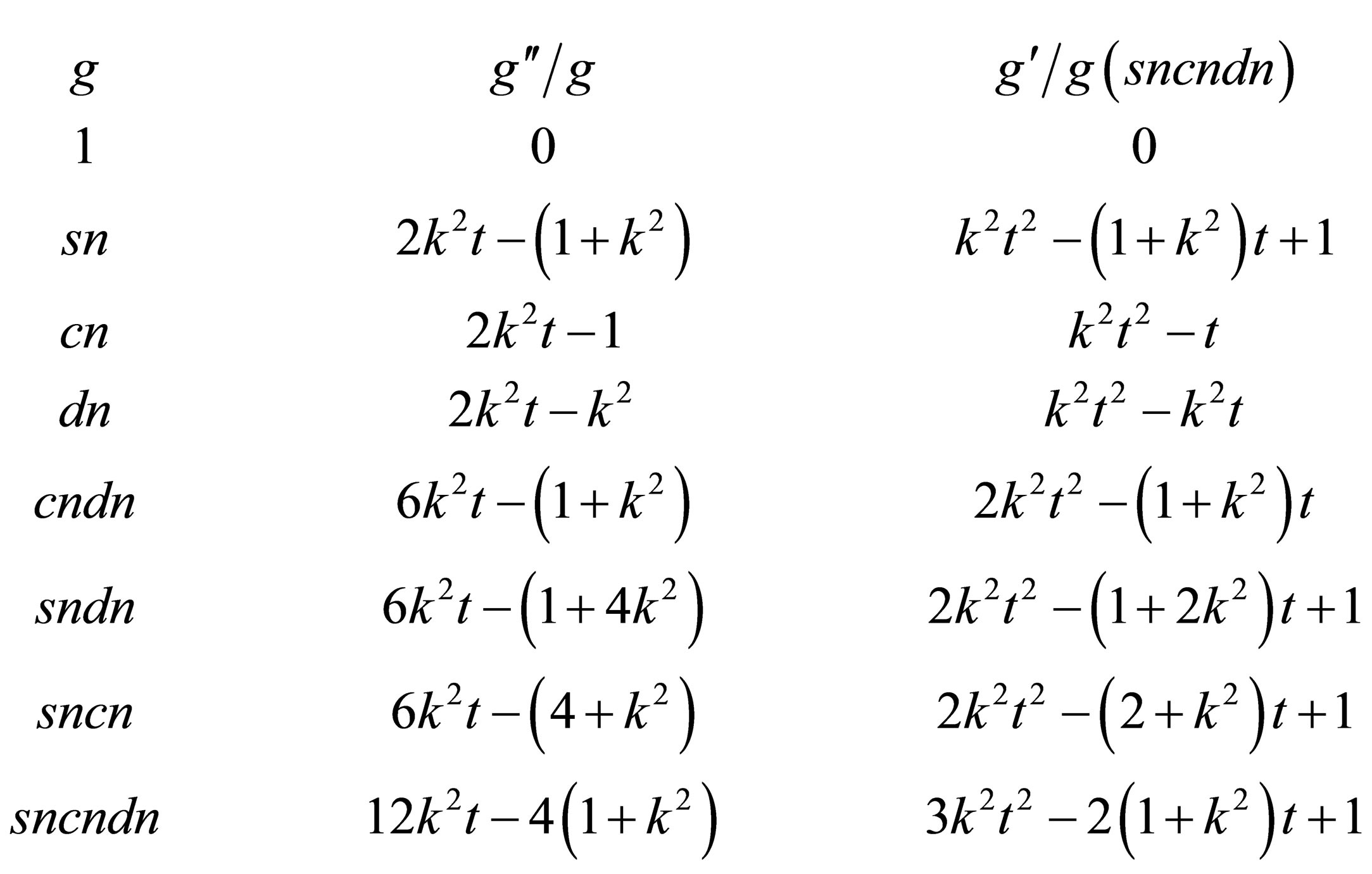
We recall that for generic values of , the Jacobi functions obey the following relations [11]:
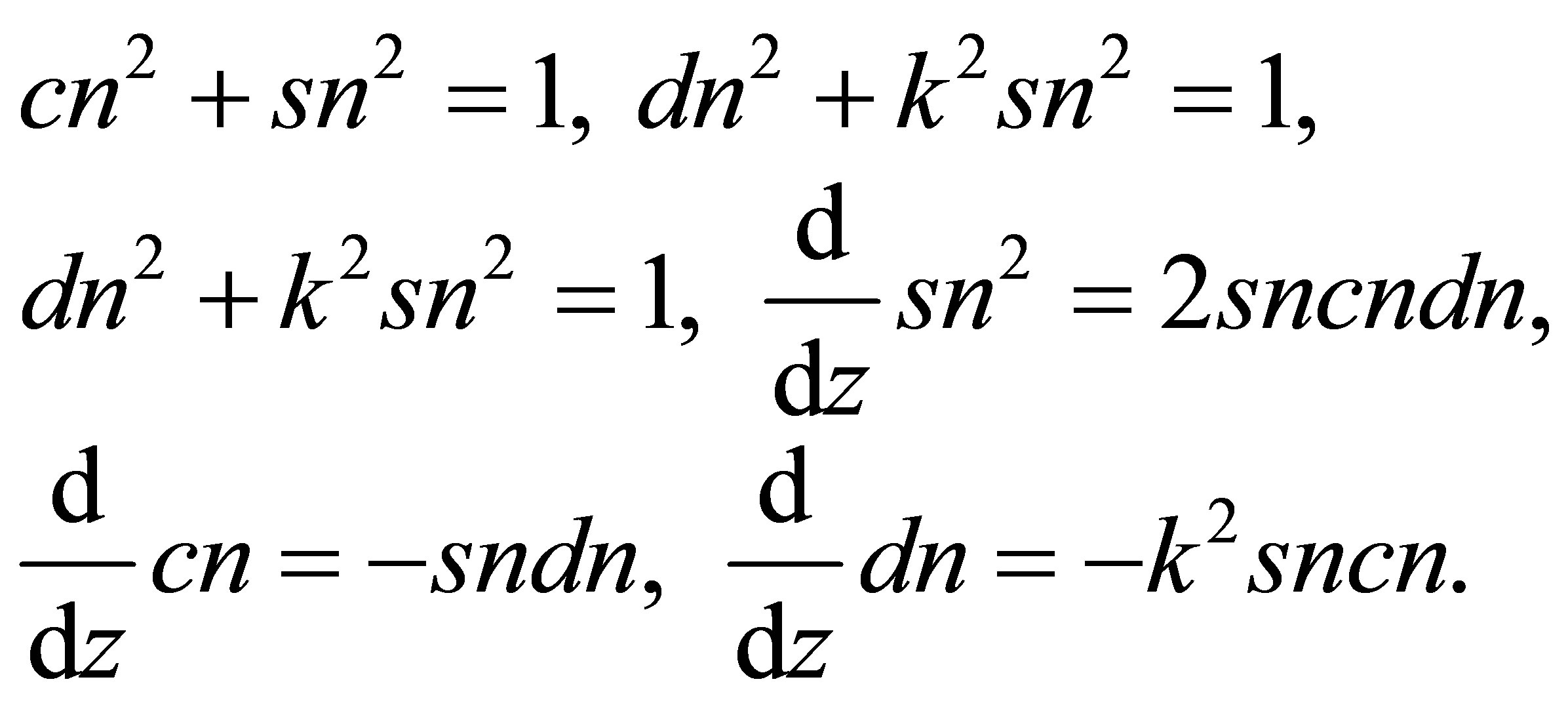 (12)
(12)
These identities as well as the following ones are useful to establish the gauge Hamiltonian (8) in the variable  after the prefactor including the Jacobi functions has been extracted [11]:
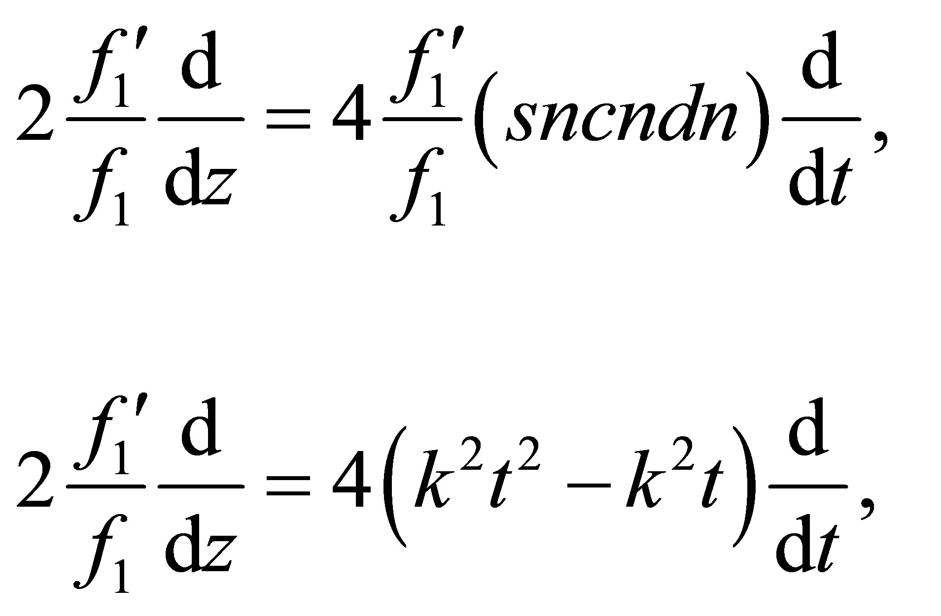
Referring to the above relations (12) and (13), for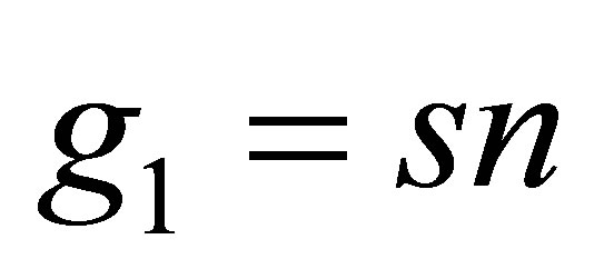 , the second term and the third term of the operator
  of the Equation (9) are written as follows:
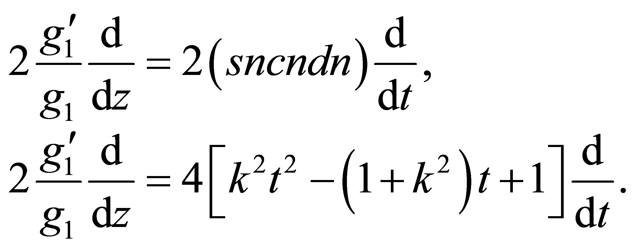 (14)
(14)
 . (15)
Referring to the same relations used previously, for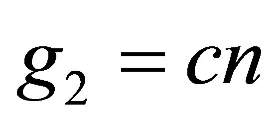 , the second term and the third term of the operator
  of the Equation (9) are of the following form:
 (16)
(16)
 . (17)
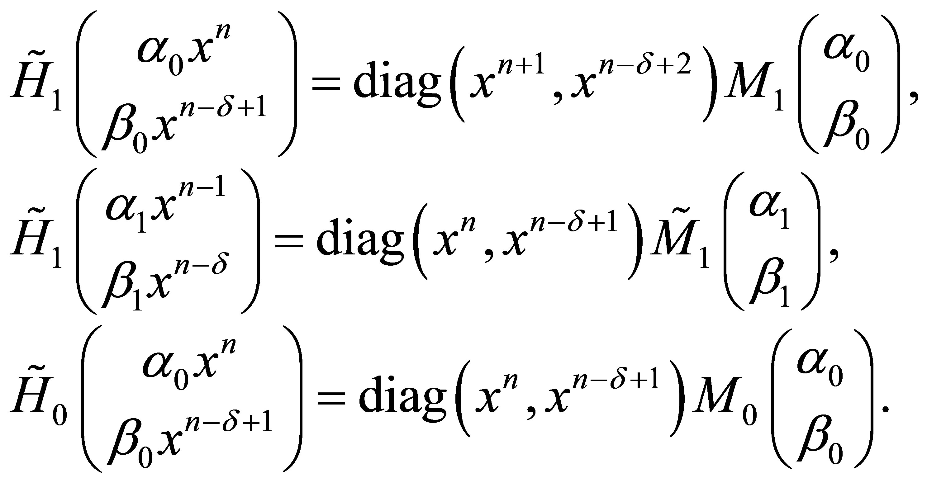
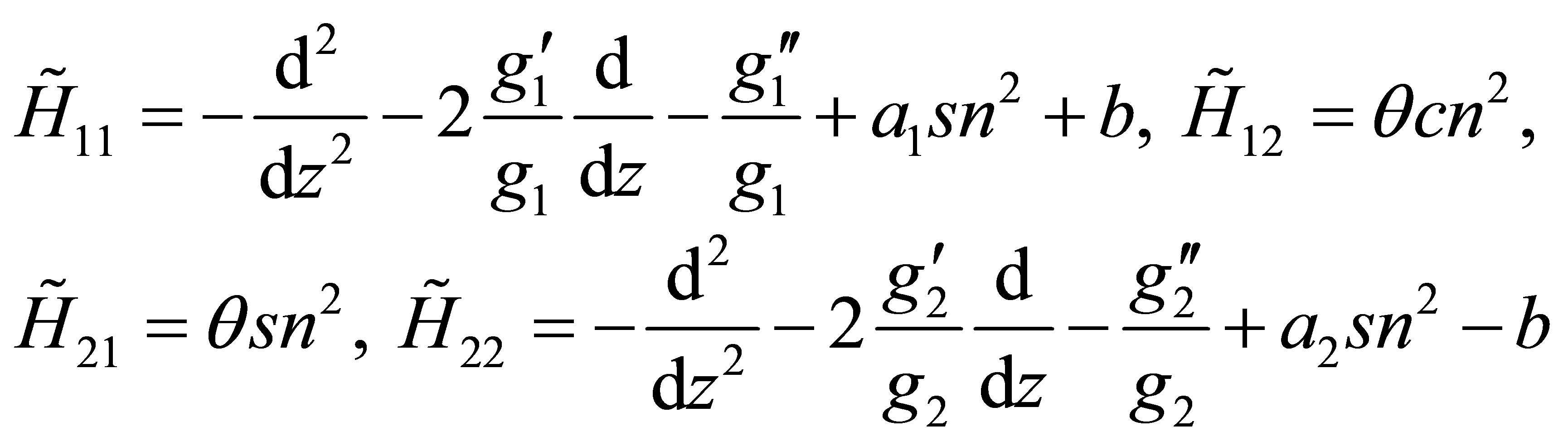
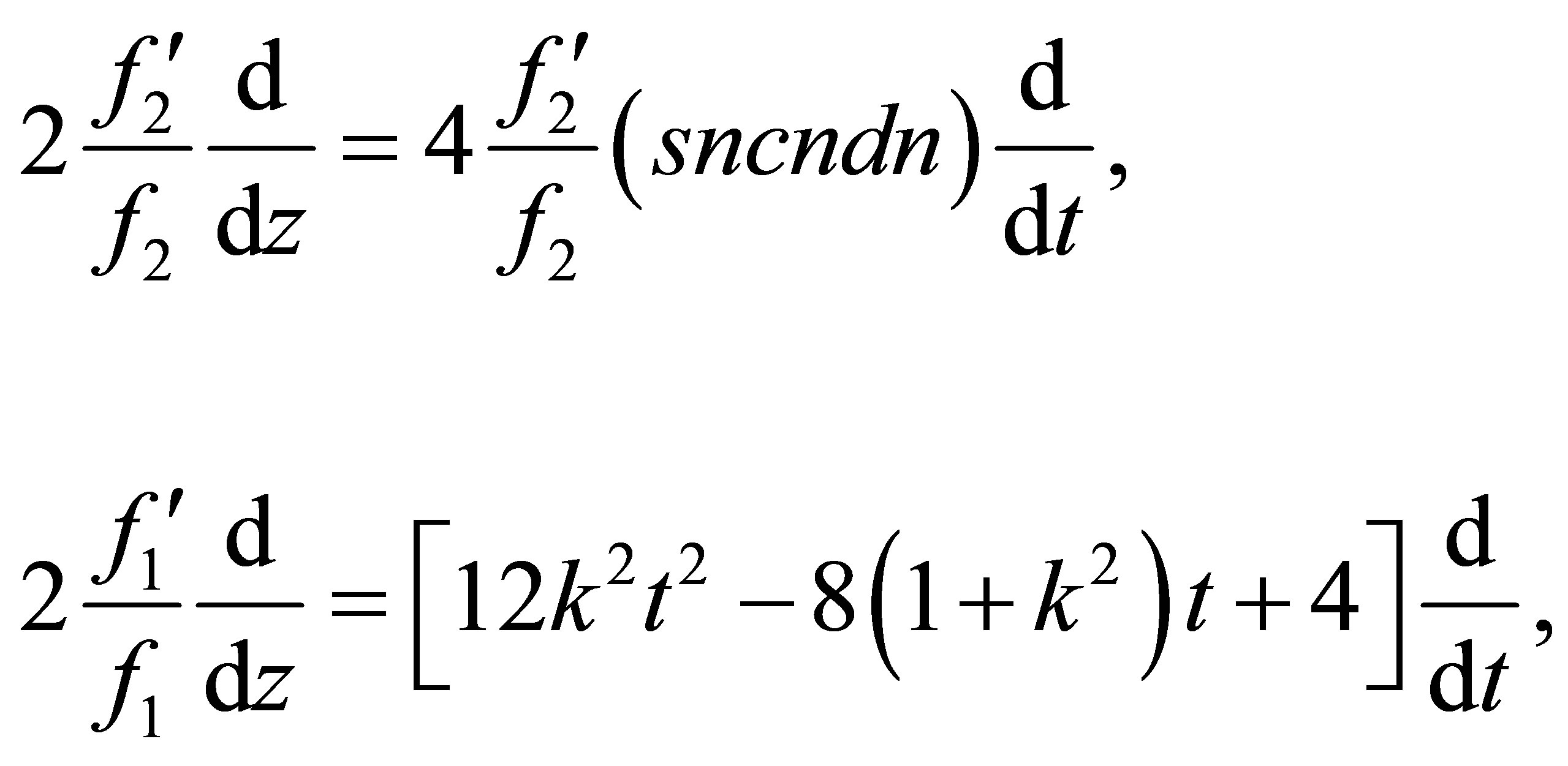
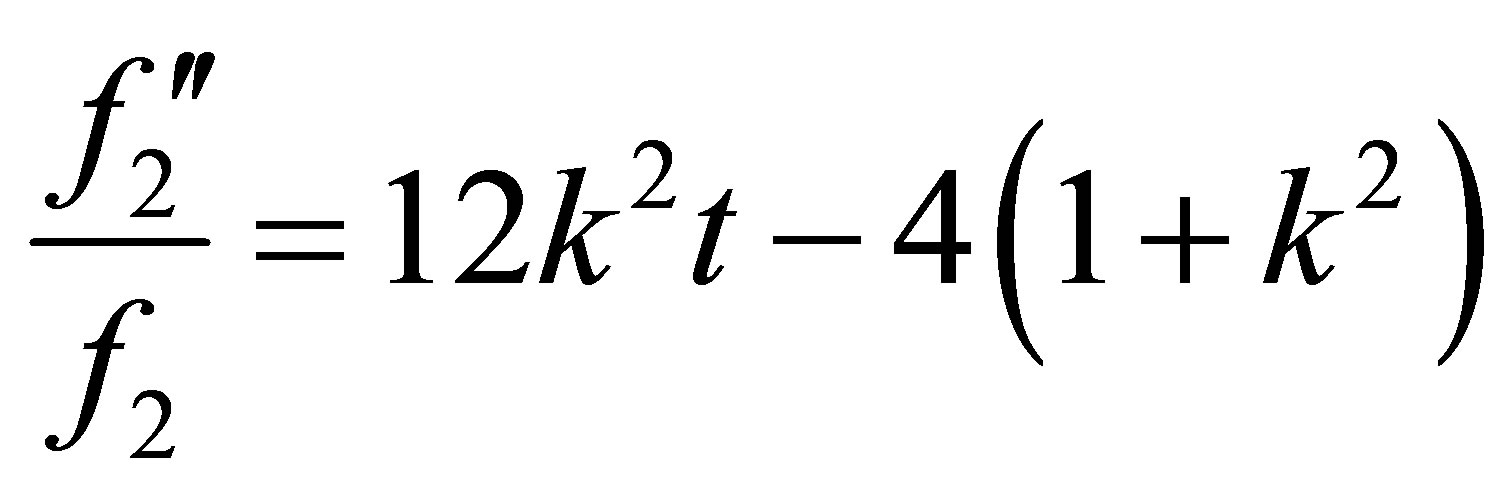
Replacing the terms of the components of the Hamiltonian  given by the Equation (9) by the expressions (11), (14)-(17) and considering the change of variable
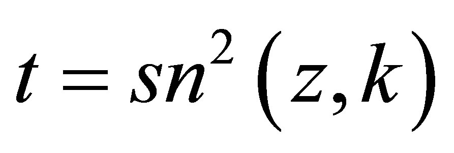 , one can easily check the following components in variable
 :
:
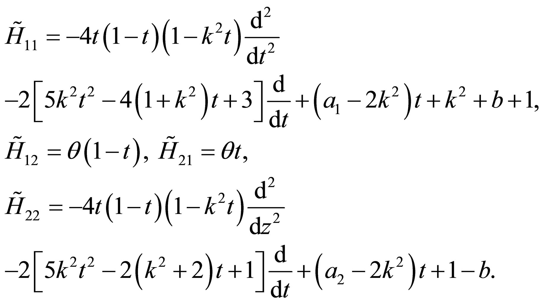 . (18)
The next step is to establish the conditions such that the gauge operator becomes quasi-exactly solvable. The so called QES conditions help to give the values of the real parameters ![]() and
and  in terms of
  and
and![]() . Indeed
. Indeed  remain free parameters and
 ![]() is an integer.
is an integer.
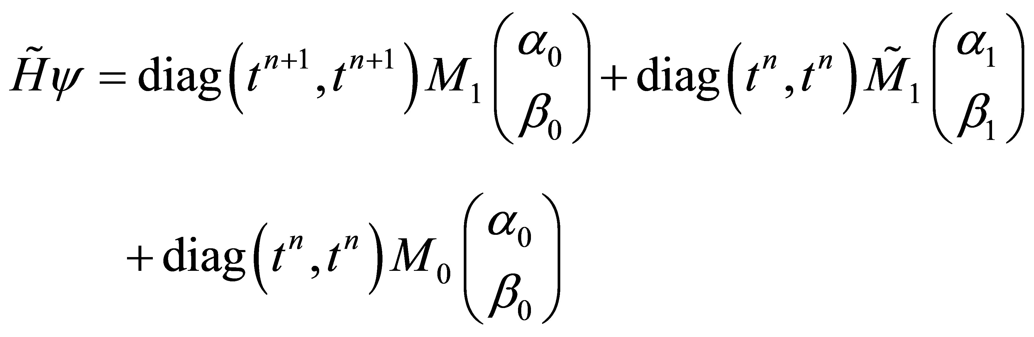
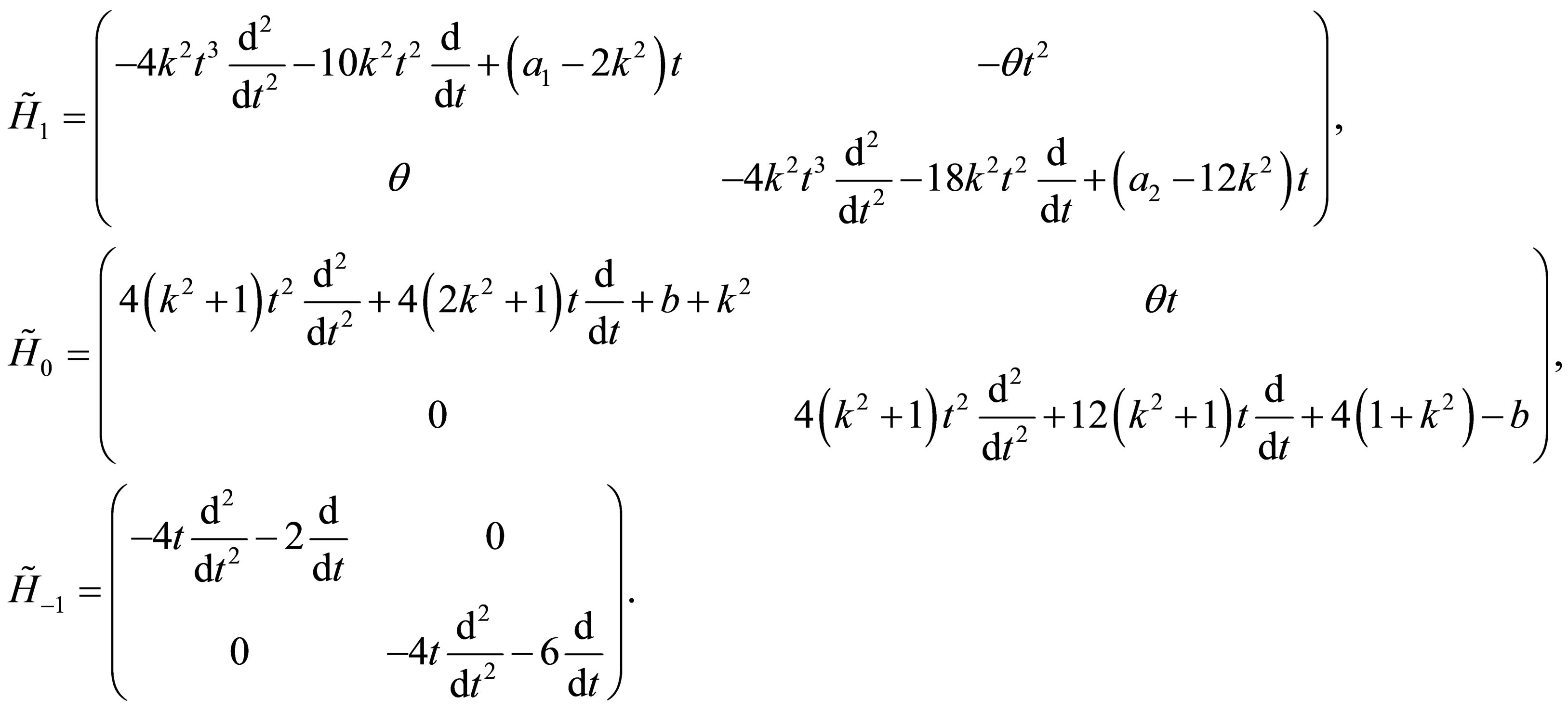
Let us decompose the operator  given by its components (18) according to
 (19)
(19)
where
| |
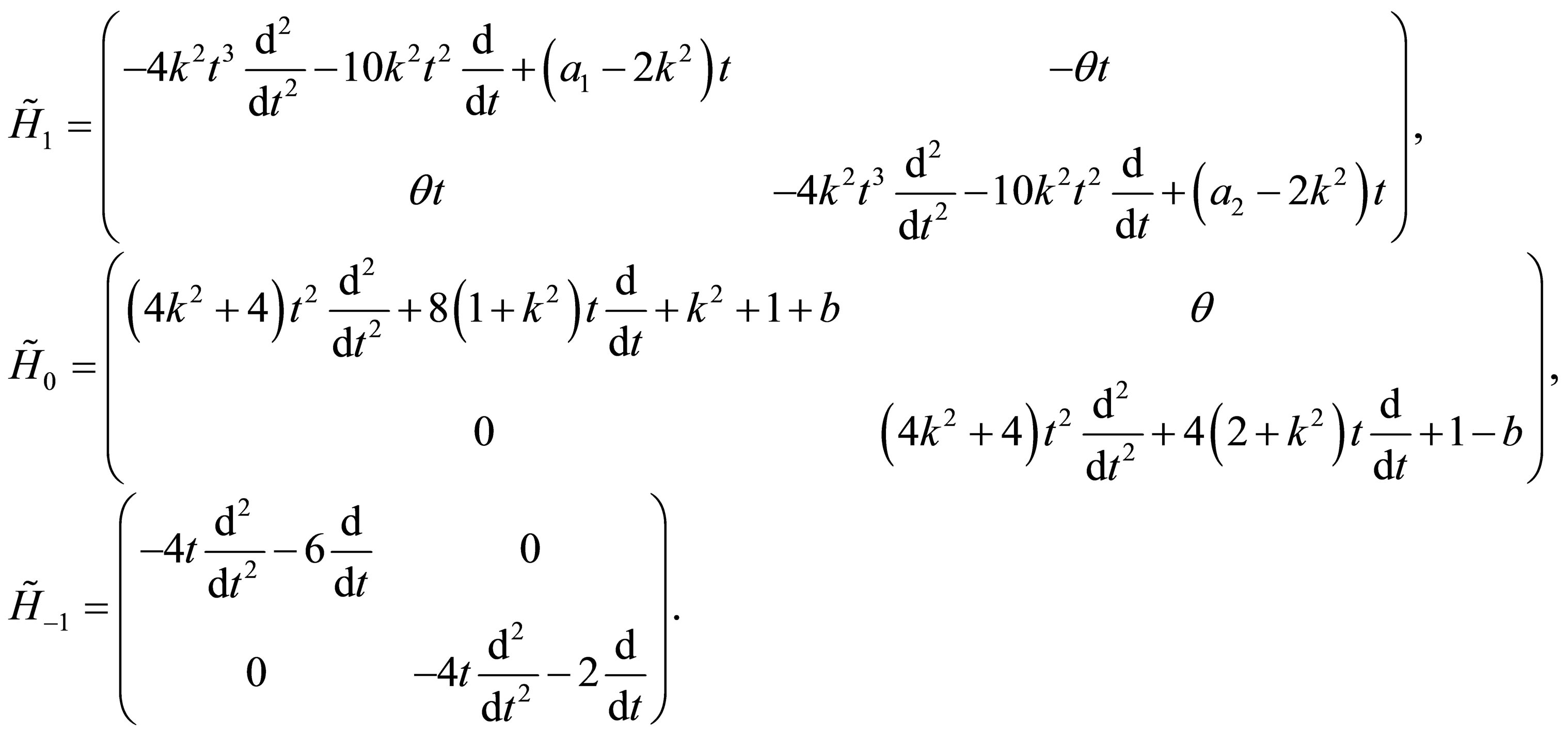 (20)
(20)
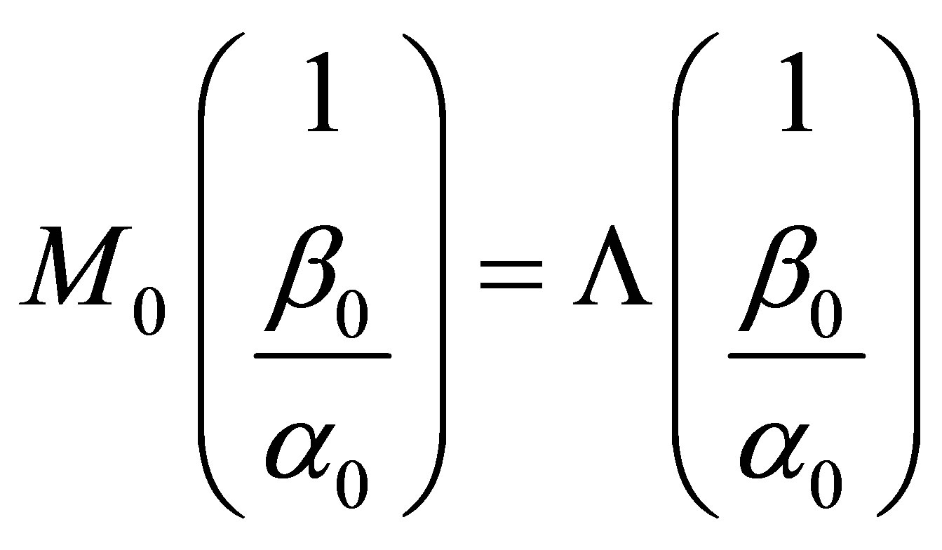
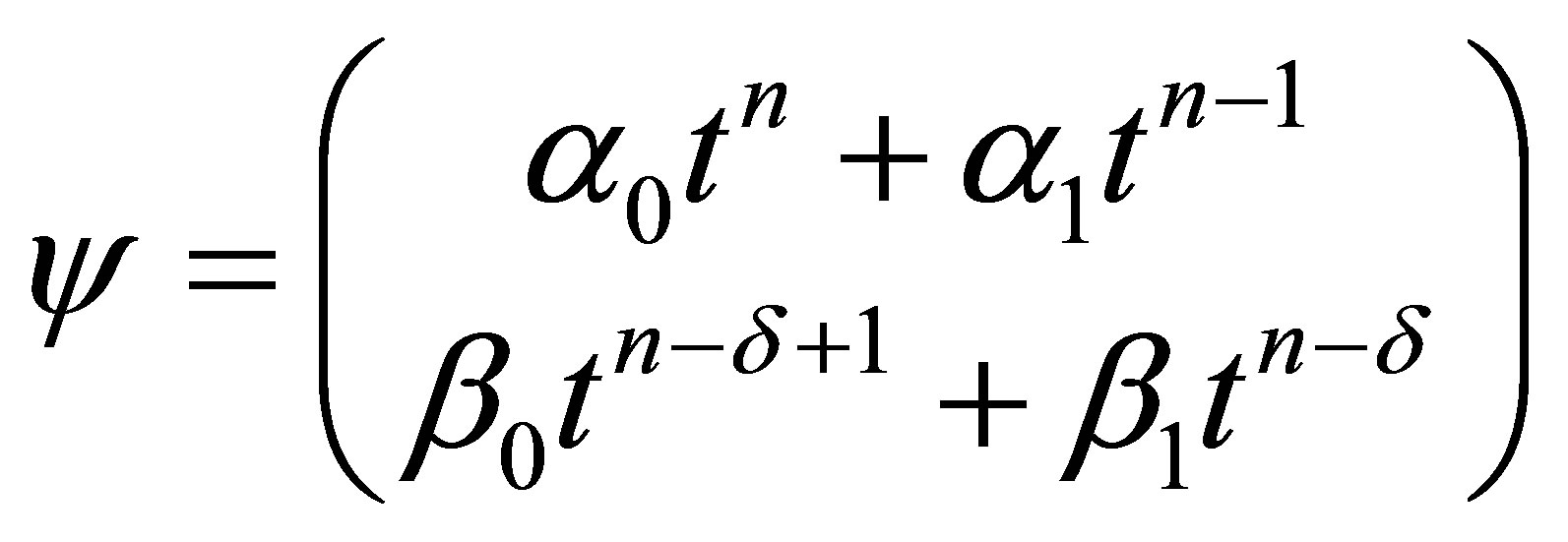
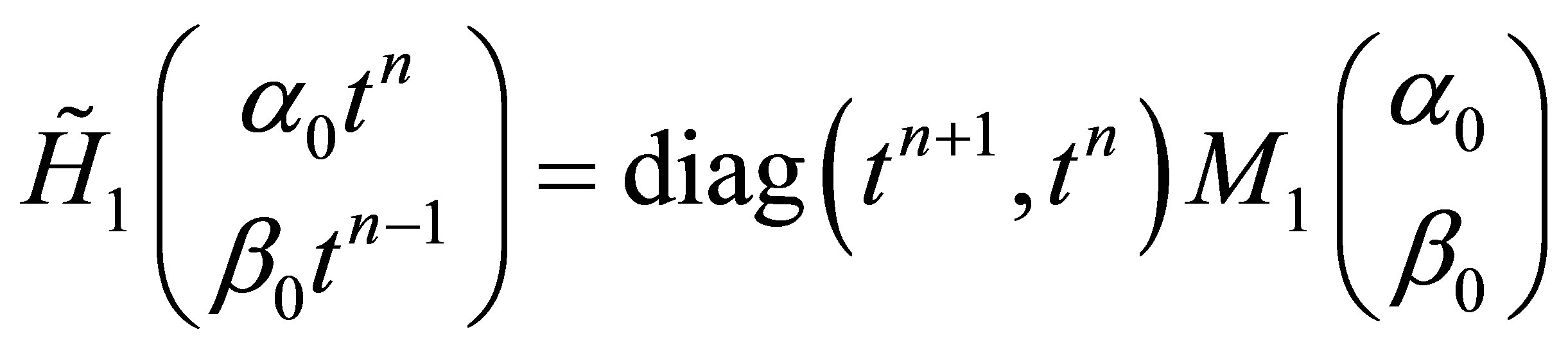
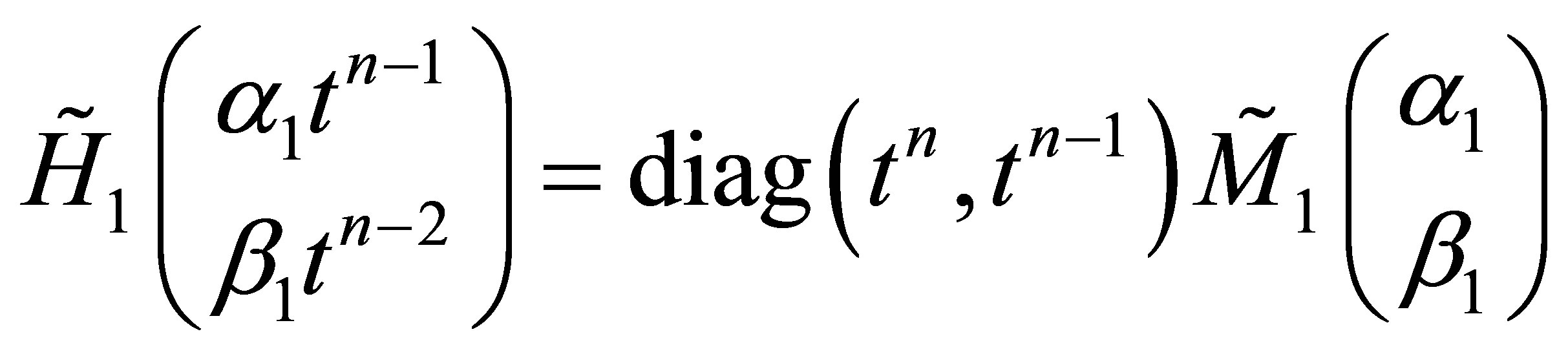
The generic vector of the invariant vector space under the action of the Hamiltonian  has the following form as it is given by the Equation (2)
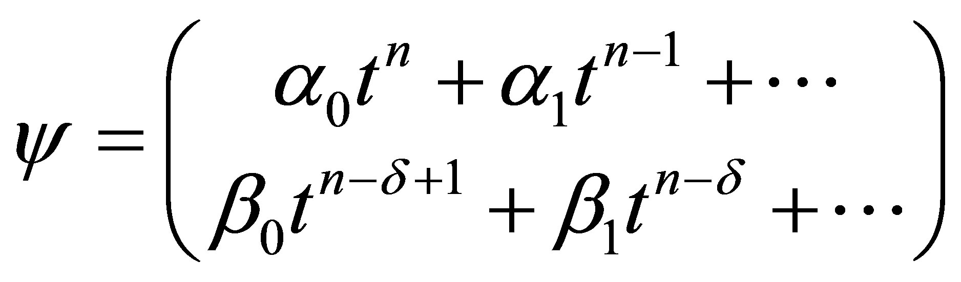
as , the above wave function
  is written as follows
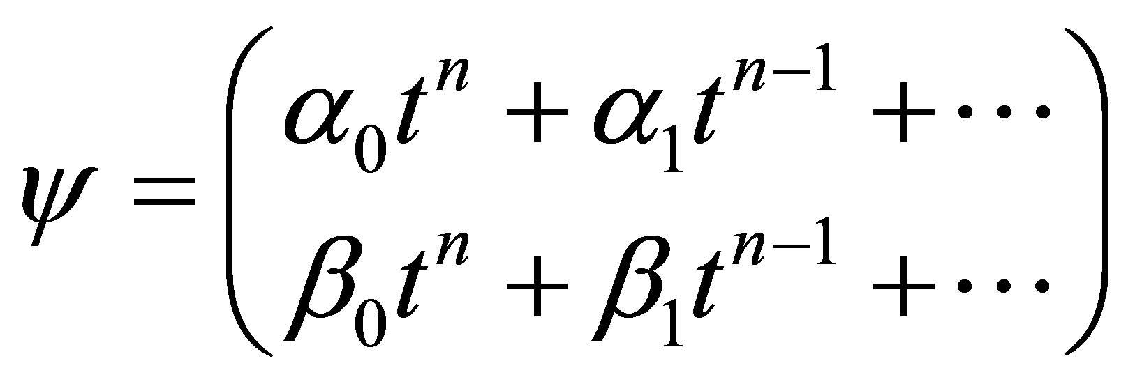 (21)
(21)
 acting on the wave function
 , he increases the degree by one unit,
 doesn’t change the degree of the wave function
 , and
, and  reduces the degree of the wave function
  by one unit.
Let the operator  acts on the above vector
 , the components of the vector
 ![]() are then polynomials in
are then polynomials in  whose components are linear in the constants
 .
.
As a consequence the vector ![]() can be decomposed uniquely according to [9]
can be decomposed uniquely according to [9]
 . (22)
This above vector defines in particular the constant 2 × 2-matrices  and
and  which are found as follows
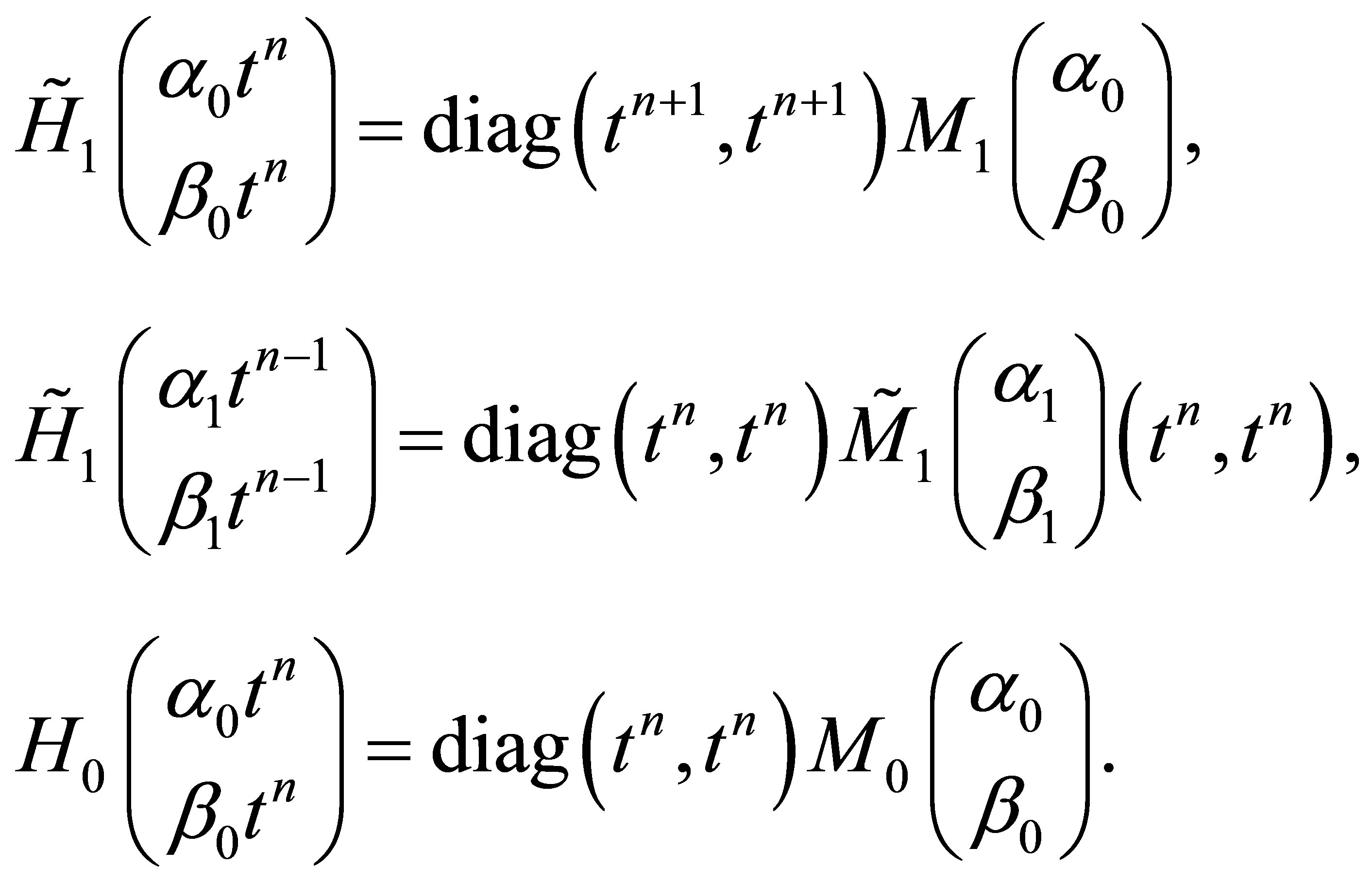 (23)
(23)
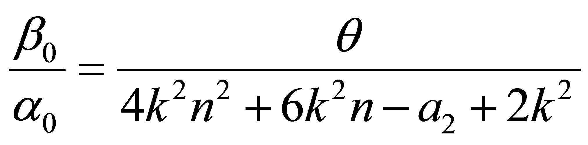
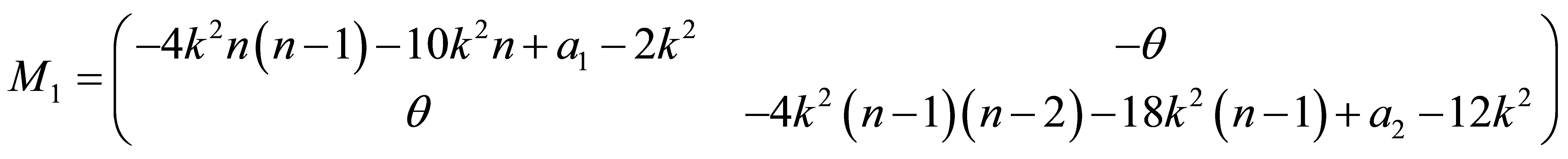
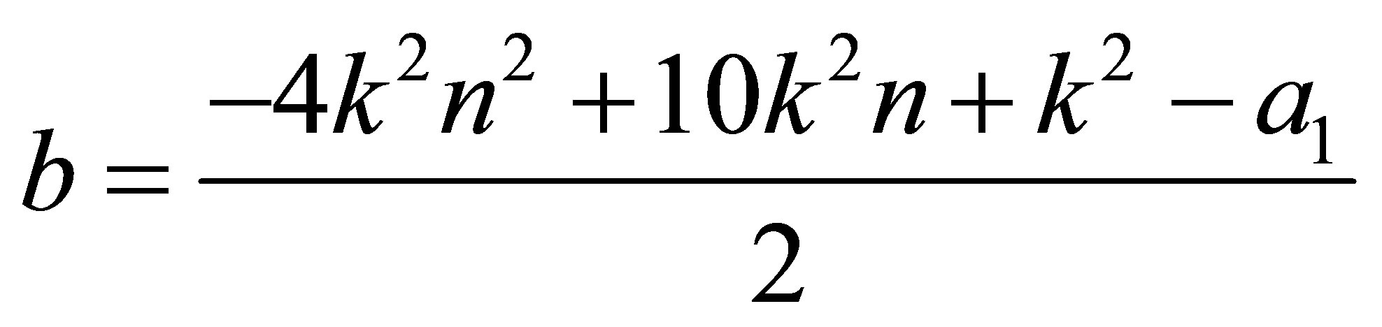
One can easily find The three necessary QES conditions for the operator  to have a finite dimensional invariant vector space are successively obtained [9]:
1) The first QES condition is
 (25)
(25)
2) the second QES condition is as follows
In this above equation replacing  by its value (25) and after some algebraic manipulations, the second QES condition is obtained
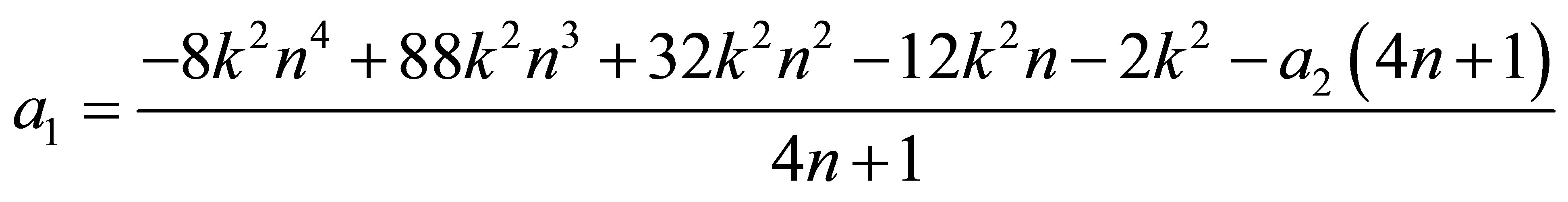 (26)
(26)
3) finally the third QES condition for the operator  to have a finite dimensional invariant vector space (i.e. the operator
  is said quasi-exactly solvable) is obtained by the condition involving the matrix
  as
as
 , (27)
| |
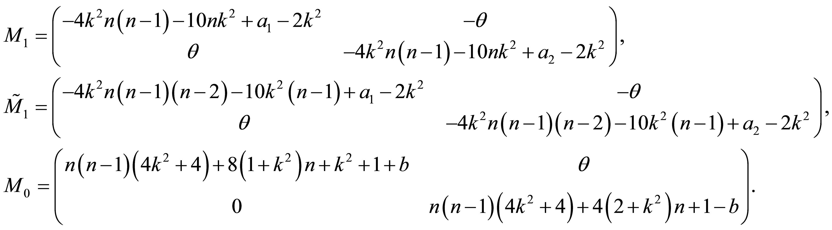
where  is a constant and
 (28)
(28)
The above expression is given by the first QES condition 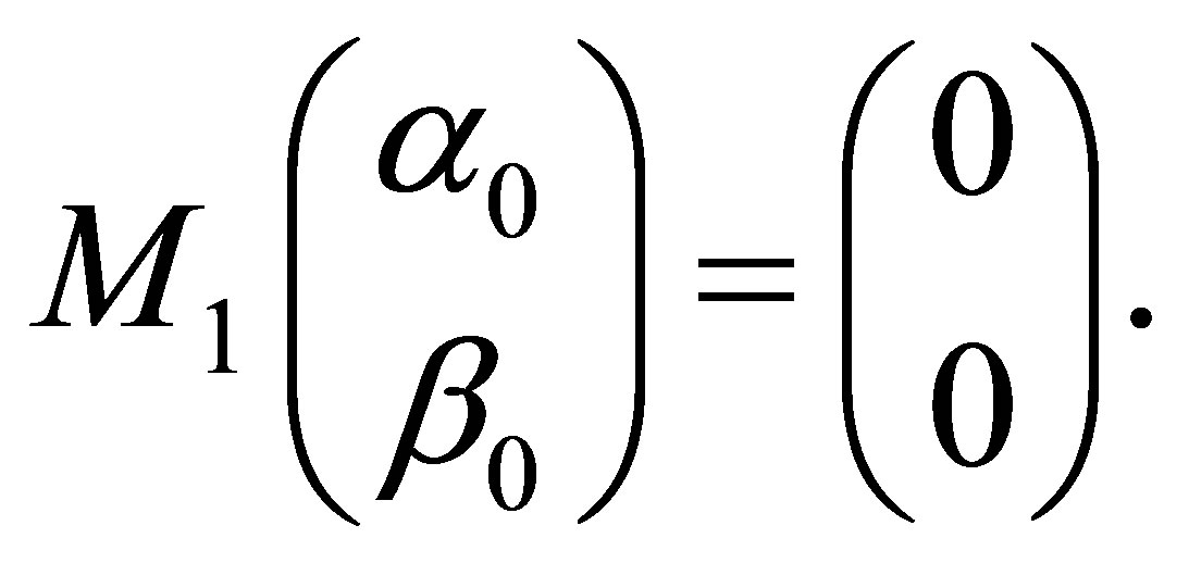
After some algebraic manipulations, the Equations (27) and (28) lead to the third QES condition
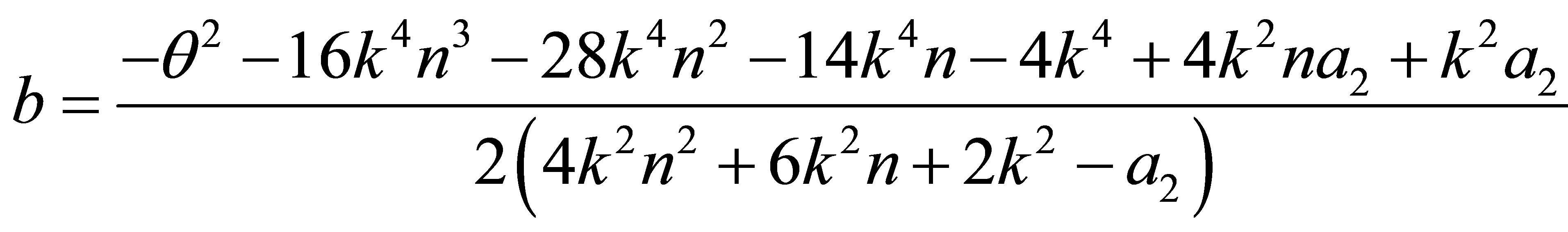 (29)
(29)
Now, referring to the QES conditions given by the Equations (25), (26) and (29), we are allowed to conclude that the operator  (therefore
 ) is quasi-exactly solvable [9]. In other words, a finite part of the eigenvalues of the operator
  can be computed algebraically. Note that the QES Hamiltonian constructed depends only on two free parameters
  and on the non negative integer
![]() .
.
3.2. Case δ = 2
Along the same lines applied for the previous case, i.e. for the case δ = 1, one has to perform a gauge transformation according to
 , (30)
after some algebraic manipulations, the components of the above Hamiltonian are of the following form
 (31)
(31)
with
and the operator  is given by the Equation (7).
Referring to the relations (12) and to the table of identities given by the Equation (13), the second term and the third term of the operator  (31) are of the following form
 (32)
(32)
 (33)
(33)
with .
.
For , the same relations (12) and the same table of identities (13) lead to the following second term and the third term of the operator
  (31):
(31):
 (34)
(34)
 . (35)
Referring to the relations (11), (32), (33), (34), (35) and after performing the change of variable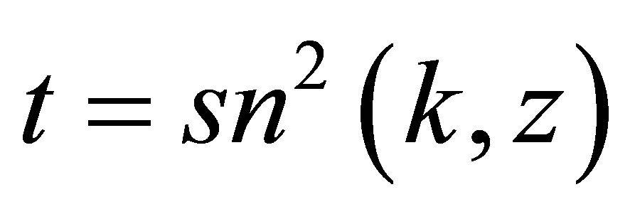 , the different components of the Hamiltonian
  given by the Equation (31) take the following form Decomposing now the above operator
  according the Equation (11), we obtain
 (36)
(36)
 (37)
(37)
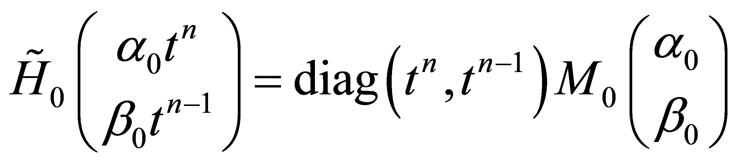
The generic element of the invariant vector space  under the action of the operator
  is given by the Equation (2) as in the QES analytic method

 the case
  leads to
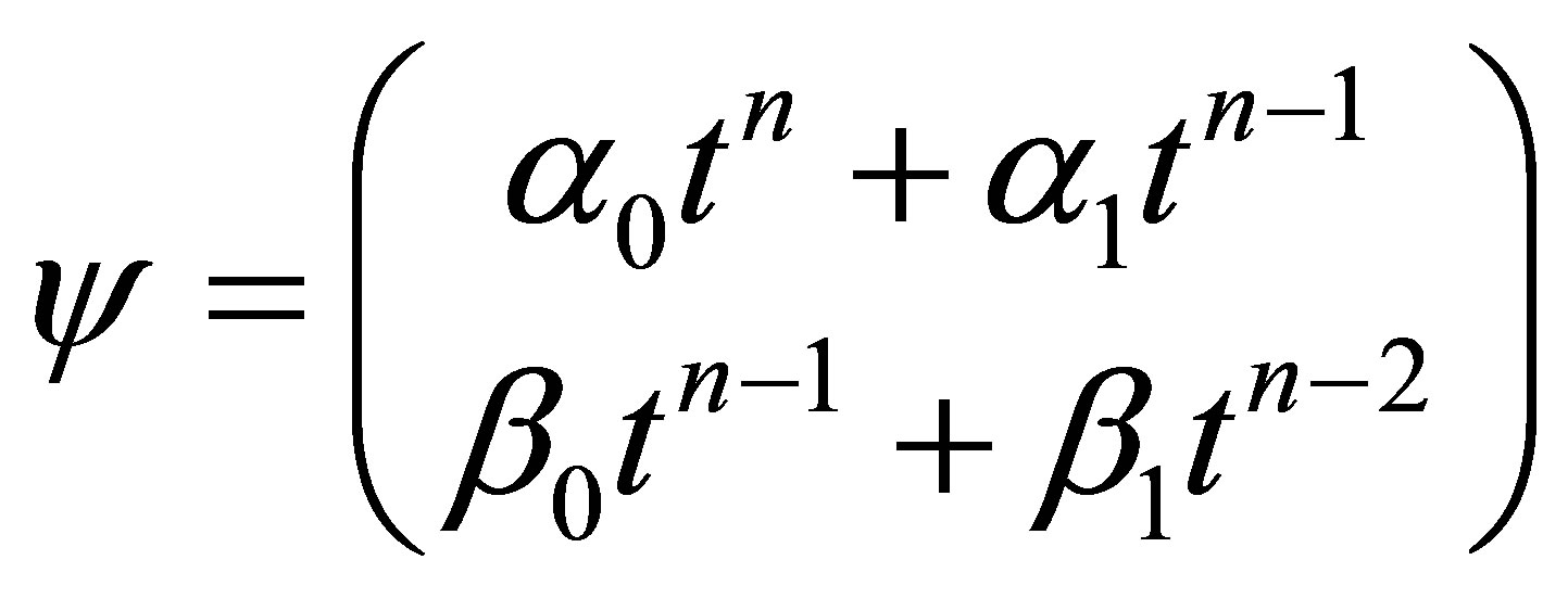 . (38)
Notice that the above operators  and
and  given by the Equations (37) are respectively the matrix operators which increases, preserves and reduces the degree of the above generic vector
  given by the Equation (38). As a consequence the vector
 ![]() can be decomposed as follows
can be decomposed as follows
 (39)
(39)
where the constant 2 × 2-matrices  and
and  can be computed explicitly after a straightforward calculation
 where
where
One can deduce the matrix 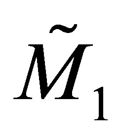 from the following expression
 where
where

finally the matrix  is easily found by
 where
where

Along the same lines used in the QES analytic method, the three necessary conditions (4) for the operator  whose components are given by the Equation (36) to be quasi-exactly solvable are successively obtained:
1) the first QES condition is as follows

2) the second QES condition is easily checked

3) Finally the third QES condition is found
 (40)
(40)
4. Conclusion
In this paper, we have applied the QES analytic method established in the Ref. [9] in order to construct a 2 × 2-matrix QES Hamiltonian which is associated to a potential depending on the Jacobi elliptic functions. We have considered two cases: 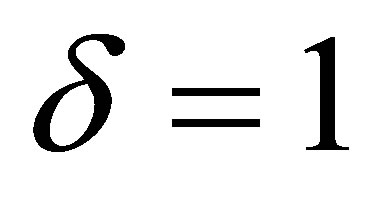 and
and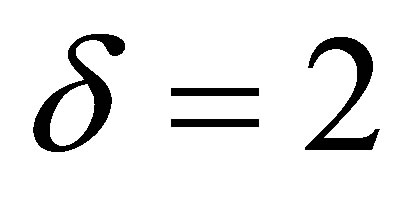 . More precisely, the three QES conditions for the Jacobi Hamiltonian to have an invariant vector space are computed algebraically.
5. Acknowledgements
I thank Pr. Yves Brihaye for useful discussions.
REFERENCES
- A. V. Turbiner, “Quasi-Exactly-Solvable Problems and sl(2) Algebra,” Communications in Mathematical Physics, Vol. 118, No. 3, 1988, pp. 467-474. doi:10.1007/BF01466727
- A. G. Ushveridze, “Quasi-Exactly Solvable Models in Quantum Mechanics,” Institute of Physics Publishing, 1995.
- A. V. Turbiner, “Lame Equation sl(2) Algebra and Isospectral Deformations,” Journal of Physics A: Mathematical and General, Vol. 22, 1989, pp. 1-144. doi:10.1088/0303-4470/22/1/001
- M. A. Shifman and A. V. Turbiner, “Quantal Problems with Partial Algebraization of the Spectrum,” Communications in Mathematical Physics, Vol. 126, No. 2, 1989, pp. 347-365. doi:10.1007/BF02125129
- A. González-López, N. Kamran and P. J. Olver, “Normalizability of One-Dimensional Quasi-Exactly Solvable Schrödinger Operators,” Communications in Mathematical Physics, Vol. 153, No. 1, 1993, pp. 117-146. doi:10.1007/BF02099042
- A. González-López, N. Kamran and P. J. Olver, “QuasiExactly Solvable Lie Algebras of Differential Operators in Two Complex Variables,” Journal of Physics A, Vol. 24, No. 17, 1991, p. 3995. doi:10.1088/0305-4470/24/17/016
- R. Zhdanov, “Quasi-Exactly Solvable Matrix Models,” Physics Letters B, Vol. 405, No. 3-4, 1997, pp. 253-256. doi:10.1016/S0370-2693(97)00655-2
- Y. Brihaye and P. Kosinski, “Quasi Exactly Solvable Matrix Models in sl(n),” Physics Letters B, Vol. 424, No. 1-2, 1997, pp. 43-47. doi:10.1016/S0370-2693(98)00167-1
- Y. Brihaye, A. Nininahazwe and B. P. Mandal, “PTSymmetric, Quasi-Exactly Solvable Matrix Hamiltonians,” Journal of Physics A: Mathematical and Theoretical, Vol. 40, No. 43, 2007, pp. 13063-13073 doi:10.1088/1751-8113/40/43/014
- Y. Brihaye and A. Nininahazwe, “Extended JaynesCummings models and (Quasi)-Exact Solvability,” Journal of Physics A: Mathematical and Theoretical, Vol. 39, No. 33, 2006, pp. 1-14. doi:10.1088/0305-4470/39/31/011
- Y. Brihaye and B. Hartmann, “Quasi-Exactly Solvable N × N-Matrix Schrödinger Operators,” Modern Physics Letters A, Vol. 16, No. 29, 2001, pp. 1895-1906. doi:10.1142/S0217732301005242
- Y. Brihaye and M. Godard, “Quasi Exactly Solvable Extensions of the Lamé Equation,” Journal of Mathematical Physics, Vol. 34, No. 11, 1993, p. 5283. doi:10.1063/1.530304