Open Journal of Microphysics
Vol. 2 No. 2 (2012) , Article ID: 19226 , 6 pages DOI:10.4236/ojm.2012.22002
Inconsistency of Probability Density in Quantum Mechanics and Its Solution
Laboratory of Theoretical Physics and Natural Phylosophy, Physics Departement, Faculty of Mathematics and Natural Sciences, Institut Teknologi Sepuluh Nopember, Surabaya, Indonesia
Email: {purwanto, b_anang}@physics.its.ac.id, eny09@mhs.physcs.its.ac.id
Received February 1, 2012; revised April 10, 2012; accepted April 19, 2012
Keywords: Schrodinger Equation; Probability Density; Particle Conservation
ABSTRACT
Probability density and particle conservation in quantum mechanics are discussed. The probability density has inconsistency with particle conservation in any quantum system. The inconsistency can be avoided by maintaining conservation of particle. The conservation coerces, a system should exist in a linear combinations of some eigenstates except ground state. The point is applied to the three exactly solvable quantum systems i.e. a particle in one dimensional well potential, harmonic oscillator and hydrogen atom.
1. Introduction
Quantum mechanics is one of the greatest scientific achievements in 20th century. In the present state of scientific knowledge, quantum mechanics plays a fundamental role in the description and understanding of natural phenomena. In fact, phenomena which occur on a very small (atomic or subatomic) scale cannot be explained outside the framework of quantum physics. For example, the existence and the properties of atoms, the chemical bond and the propagation of an electron in a crystal cannot be understood in terms of classical mechanics.
Even when we are concerned only with macroscopic physical objects (that is, whose dimensions are comparable to those encountered in everyday life), it is necessary, in principle, to begin by studying the behavior of their various constituent atoms, ions, electrons, in order to arrive at a complete scientific description. There are many phenomena which reveal, on a macroscopic scale, the quantum behavior of nature. It is in this sense that it can be said that quantum mechanics is the basis of our present understanding of all natural phenomena.
Quantum mechanics became a wonderful and extremely powerful tool. The properties of the different materials, the whole chemistry, became for the first time objects that could be predicted from the theory and not only phenomenological rules deduced from experiments. The technological discovery that shaped the second half of the last century, the transistor as the basis of all the modern electronics and computers, could not be invented without a deep command of quantum mechanics.
Recently, quantum mechanics leads to the possibility of constructing a quantum computer that would improve the speed of present day computers by an incredible factor [1]. Another possible practical application is quantum cryptography [2], in which a message is transmitted in such a way that it cannot be read without interfering with it. Another quantum-information puzzling phenomenon, the teleportation [3], has been recently proved experimentally to exist and it is a very active area of experimental research.
In spite of the above remarkable successes, quantum mechanics remains mysterious, although each year it is taught in thousands of university courses. It is not only the problem of explaining its meaning without using advanced mathematics that forbids a simple exposition of its properties to the layman. One can read and follow a comprehensive description all of the problem of the foundation of quantum mechanics and a deep interpretation of quantum mechanics in a unique book of Auletta [4]
Not all of the problem of foundation and interpretation of quantum mechanics is explained in standard textbooks of the subject. One foundation which is always introduced in textbook of quantum mechanics is probability density. The fundamental objects in quantum mechanics are complex amplitudes and probabilities are the modulus square.
Probability was not unknown in physics. It was introduced by Boltzmann in order to control the behavior of a system with a very large number of particles. It was the missing concept in order to understand the thermodynamics of macroscopic bodies, but the structure of the physical laws remained still deterministic. The introducetion of probability was needed as a consequence of our lack of knowledge of the initial conditions of the system and our ability to solve an enormous number of coupled nonlinear differential equations. If we were both infinitely able experimentalists and infinitely able mathematicians, probability would be useless in classical physics: it is only a tool which allows imperfect beings, with a bounded brain like us, to control the behavior of many particle systems.
In quantum mechanics, the tune is different: if we have 106 radioactive atoms there are no intrinsic unknown variables decide which of them will decay firstly. What we observe experimentally seems to be an irreducible random process. The original explanation of this phenomenon in quantum mechanics was rather unexpected. All atoms have the same probability of having decayed: only when we observe the system we select which atoms have decayed in the past. In spite of the fact that this solution seems to be in contrast with common sense, it is the only possible one in the framework of the conventional interpretation of quantum mechanics.
In this paper, we investigated the probability density and have discovered its inconsitency for all quantum mechanical systems which can be solved analytically. We can find, for example, in standart textbooks of quantum mechanics for examples, [5-9]. The inconsistency between concept and physical interpretation of probability density may give rise confusion for students and readers in general. The inconsistency can be avoided by maintaining conservation of particle. The conservation coerces, a system should exist in a linear combinations of some eigenstates except ground state.
The article is organized as follows. Section 2 gives short review on the Schrodinger equation and continuity equation. Section 3 describes probability density of three analytical solvable quantum mechanical systems i.e. particle in infinite potential well, particle in oscillator harmonics potential and electron in hydrogen atom. Finally, discussions and conclusions, presenting how to solve the inconsitency of probility density problem, are given in Section 4.
2. Probability Density
2.1. Schrodinger Equation
Quantum mechanics was discovered twice: first, by Werner Heisenberg in 1925 as matrix mechanics [10], and then again by Erwin Schrodinger in 1926 as wave mechanics [11-13]. The two forms were soon found to be identical in content, but wave mechanics is used more intensively as approach to introduce the concepts of quantum mechanics in the associated textbooks and became more useful tool because the mathematics of waves were more familiar than matrix mechanics.
At the very beginning of the development of quantum mechanics, one was faced with the problem of finding a differential equation describing discrete state of an atom. It was not possible to deduce exactly such an equation from old and well known physical principles; instead, one had to search for parallels, in classical mechanics and try to deduce the desired equation on the basis of plausible arguments. Such an equation, not derived but guessed at intuitively, would then be a postulate of the new theory, and its validity would have to be checked by experiment. This equation for the calculation of quantum-mechanical states is called the Schrodinger equation. Short and fine qualitatively review obtaining Schrodinger equation was given in old textbook of Schiff [7].
At the end of the nineteenth century, people distinguished between two entities in physical phenomena: matter and radiation. Completely different laws were used for each one. The laws of Newtonian mechanics were utilized to predict the motion of material bodies. With regard to radiation, the theory of electromagnetism, thanks to the introduction of Maxwell’s equations, had produced a unified interpretation of a set of phenomena of radiation, which had previously been considered as belonging to different domains: electricity, magnetism and optics.
Quantum ideas contributed to a remarkable unification of the concepts of fundamental physics by treating material particles and radiation on the same footing. Different from classical one, wave equation of quantum mechanics contains a first derivative with respect to t and a second derivative with respect to x
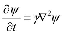 (1)
(1)
Phase of wave exp (ikr - iwt) and relation between energy and momentum of a free particle E = p2/2m lead to wave equation
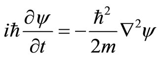 .(2)
.(2)
The parameters of particle (the energy E and the momentum p of a photon) and wave parameters (the angular frequency w and the wave vector k) are linked by the fundamental relations E = ħw and p = ħk. Simply, wave Equation (2) seems as if transition from energy and momentum to differential operators
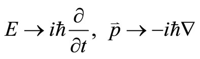 ,(3)
,(3)
then operate to a wave function ψ.
The extension from the free-particle wave Equation (2) so that it includes the effects of external forces that may act on the particle may be done directly. We shall assume for the present that these forces are of such a nature (electrostatic, gravitational, possibly nuclear) that they can be combined into a single force F that is derivable from a potential energy V,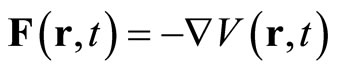 . The total energy for system of particle with mass m and momentum within the region with potential V consist of kinetic energy and potential energy is expressed as Hamiltonian
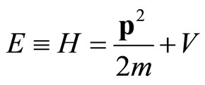 (4)
(4)
After substitution of the differential operators, Equation (3), and operating on wave function ψ(r,t), one obtain the three-dimensional Schrodinger equation
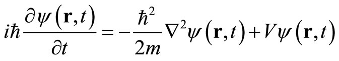 (5)
(5)
The solution of this equation, wave function ψ(r,t), should provide a quantum-mechanically complete description of the behavior of an particle of mass m with the potential energy V(r,t).
In a case of the potential V does not depend on time, the Schrodinger Equation (14) is reduced to a form
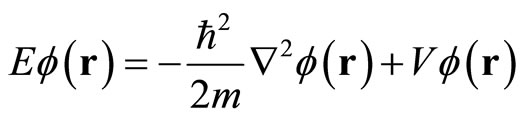 (6)
(6)
This is the time independent Schrodinger equation. The time dependent wave function ψ(r,t) is related with time independent wave function φ(r) according to
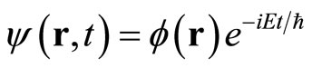 (7)
(7)
2.2. Continuity Equation and Copenhagen Interpretation
The ultimate justification for choosing Equation (5), must, of course, come from agreement between predictions and experiment. The solution of Schrodinger Equation (5), wave function ψ(r,t), is assumed to contain all information about the state of the physical system at time t.
In general, ψ(r,t) is a complex function, has no physiccal meaning and cannot be a direct measure of the likelyhood of finding a particle at position r at time t. The positive quantity  measures the probability of finding a particle in the vicinity of r at time t. This probability interpretation is due to Max Born who, shortly after the discovery of the Schrodinger equation, studied the scattering of a beam of electrons by a target, and was explained in almost all textbooks of quantum mechanics. For example, in one dimensional case, the probability of finding electron, described by a wave function ψ(x,t), in the region lying between x and x + dx is given by [2]
 (8)
(8)
According to the probability interpretation, if there is a particle in space then
 .(9)
.(9)
In the classical quantum mechanics, it is assumed that a particle is conserved, cannot be destroyed or annihilated as well as created. The wave function satisfying this equation is called normalized wave function.
The probability interpretation of the ψ(r,t) waves can be made consistently only if this conservation of probability is guaranteed. This requirement is fulfilled, owing to Gauss’ integral theorem, if it is possible to define a probability current density j which together with the probability density ρ = ψ*ψ satisfies a continuity equation
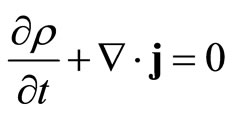 .(10)
.(10)
It is exactly as in the case of the conservation of matter in hydrodynamics, or conservation of charge in electrodynamics. In electrodynamics, this equation is the law of conservation for the electric charge: if the charge density in a volume element changes, then a current flows through the surface of the volume element (Gauss’ law).
In quantum mechanics, ρ is the probability density and after a little process one obtain the probability current density
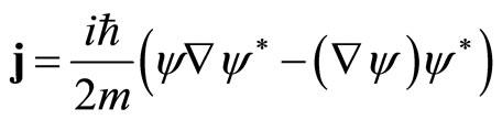 (11)
(11)
Application of Gauss’ law leads to the integrated equation
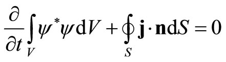 (12)
(12)
The particle flux through the surface of a region, if there is no particles be created or annihilated, is equivalent to the variation of the particle density inside the region.
3. Particle Conservation
3.1. Infinite Potential Well
The textbooks on quantum mechanics usually start with one dimensional case to illustrate some non-classical effects of the theory. The simplest one-dimensional quantum mechanical system is a particle of mass m in region with potential is zero along L and otherwise is infinite. The Schrodinger equation is given
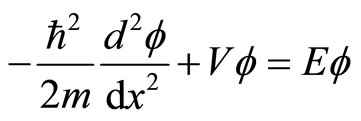 ,(13)
,(13)
with potential V = 0 for 0 ≤ x ≤ L and otherwise are infinite. The infiniteness of potential ensures that the particle mass m can’t be outside the well L. It implies that wave function vanishes outside the well and gives the boundary conditions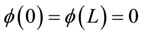 .
.
Potential V = 0 inside the well L, boundary conditions and normalization requirement, Equation (9), in onedimension
 (14)
(14)
give wave or eigen functions
 (15)
(15)
and eigen energies
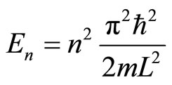 (16)
(16)
with n = 1, 2, 3, ... are called quantum numbers. Eigen energies show the first non-classical effect of quantum mechanics that is the quantum system has a discrete energy, not continue as in classical system. In this paper, we are interested in the characteristic of the probability density.
Physically, The nornalization condition, Equation (14), states that the particle of mass m definitely exists in the well L. Peculiarly, the probability of finding a particle in the region lying between x and x + dx is given by
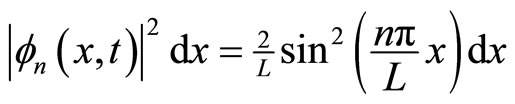 .(17)
.(17)
When the particle is at ground state, it can move freely to the right and vice versa. The particle can be found or observed at any point in the well. However, the situation will be difference when the particle is at excited state, see Figure 1.
We can see, from Figure 1, for the first excited state, φ2(x), particle can be found at left or right part in the well but never be at the center
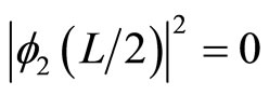 . (18)
This result gives rise inconsistency as follows.
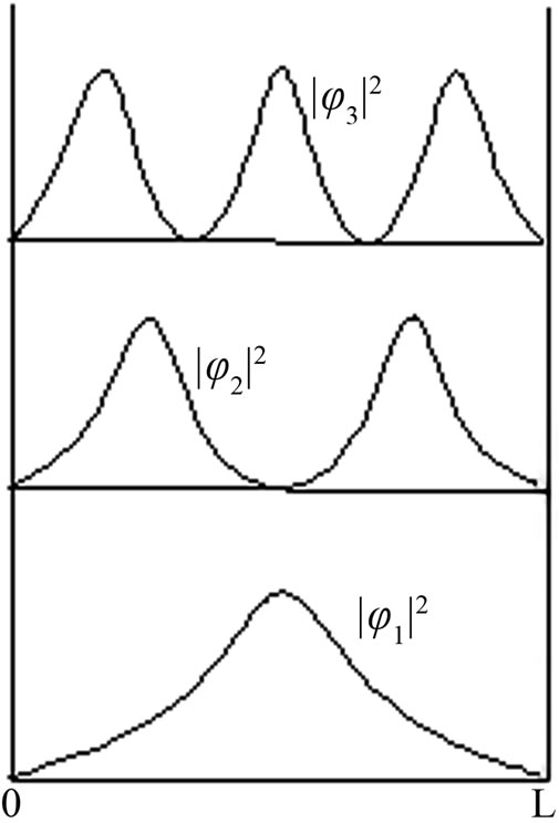
Figure 1. Probability density of a particle in the well.
If the particle always presents that is never disappear or annihilated, then the particle which is at the right or left part momentarily must move through the center of the well. It means, the probability of particle in the center is not actually zero and the result of Equation (18) is disobey. On the contrary, if particle can be annihilated while crossing at the center of well from left to right and vice versa then when the particle vanishes its density probability is zero, at the moment, at all positions in the well. When it is happened then Equation (14) is violated.
This situation occurs for all excited states, since , has n - 1 zero density probabilities at x = kL/n
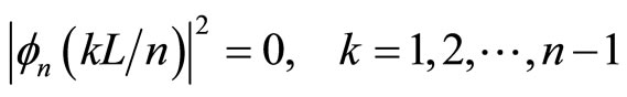 . (19)
The particle can stay at two points but never stay at a certain point among them. If the particle can exist at every point in the well, it means the particle can move freely along the well. Further, the particle can exist and be observed at all points in the well. It can be occured if there are no zero points of density probability.
3.2. Harmonic Oscillator
The next application of the Schrodinger equation is a particle in an oscillator potential. From classical mechanics we know that such a potential is of great importance, because many complicated potentials can be approximated in the vicinity of their equilibrium points by a harmonic oscillator.
The classical Hamiltonian function of a particle of mass m oscillating with frequency w takes the form
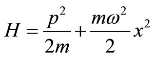 . (20)
From this Hamiltonian, one obtains the stationary Schrodinger equation of harmonic oscillator of the form
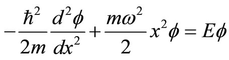 . (21)
The stationary states of the harmonic oscillator in quantum mechanics are
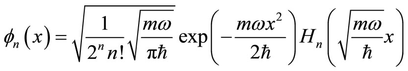 (22)
(22)
where quantum number n = 0, 1, 2, …, and Hn is Hermite polynomial whose n zero points. Energy of the particle is 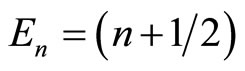 ħw.
ħw.
Some graphs of probability density Pn = |φn|2 are given by Figure 2. The situations of oscillator particle are similar with particle in well. The particle in ground state can move freely from equilibrium point to the left or right. The problem is occurred when the particle in the excited states. The n-th excited state has n zero points, one of these zero pints is at equilibrium point if n is odd. The
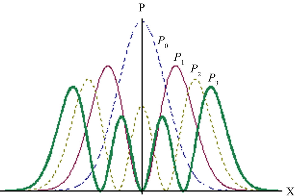
Figure 2. Probability density of particle in oscillator.
zero points imply that particle may exist at two points but never stay at certain point between them. It is, of course, impossible one if the particle can’t be annihilated and created as assumed in quantum mechanics. Then, as particle in infinite potential well, the state of oscillator particle should be linear combination of two or more eigenfunctions with totally different zero points.
3.3. Hydrogen Atom
The last quantum mechanical system we consider is hydrogen atom. Without lost generality, for simplicity we assume that an atomic nucleus is at the rest. The Schrodinger equation of hydrogen atom is given
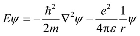 . (23)
Considering the symmetry of the system, Laplacian operator Ñ2 is given in spherical coordinate. Variable separation and finitely reasons in the zero point coordinate and vanishing function at infinitely give solution
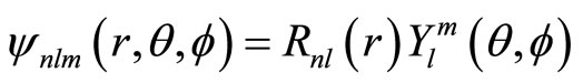 (24)
(24)
with  is spherical harmonic function and Rnl(r) is radial function. Here, we only consider radial probability. The behavior of polar probability is similar with radial probability. Several function Rnl(r) are given in Table 1 below.
The radial probability density is defined as
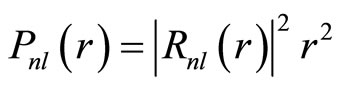 . (25)
In general, the properties of particle described by this probability are similar with previous ones. Electron is permitted to stay at some area but forbidden at some surfaces. For any Rnl(r) there are n - l peaks and n - l - 1 zero surface. For an example n = 3, the radial probability has two peaks and one zero surface, as in Figure 3.
The electron may be in a single groundstate. The different from the previous ones is the electron in hydrogen
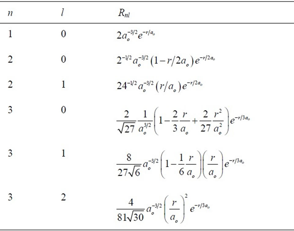
Table 1. Radial functions of hydrogen atom state functions.
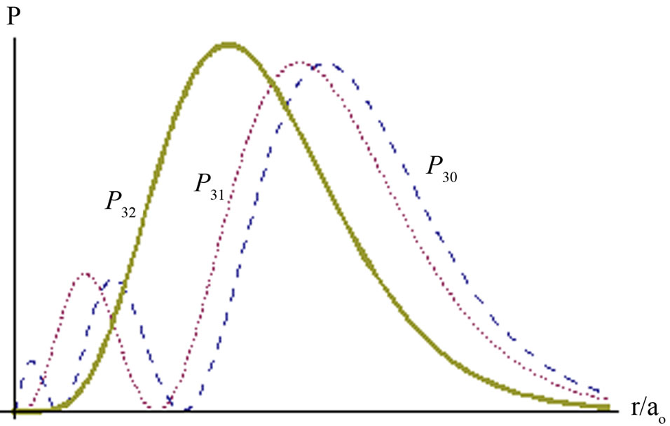
Figure 3. Radial probability P3l of electron in hydrogen atom.
atom has degeneracy states. It implies that electron may exist at single excited state Rnl(r) with n is bigger than one, as long as satisfies n - l is equal to one. Otherwise, it should be linear combination of two or more states.
4. Discussions and Conclusions
We have shown that the probability interpretation of single eigenfunction of Schrodinger equation, in general, has inconsistency with conservation of particle. To be consistent, the eigenfunctions should be in linear combinations. However, some linear combinations are not allowed. The details are as follows.
The particle in potential well or oscillatory potential may be at single eigen state only when the state is ground state. However, in case of hydrogen atom, the electron may be in single state although it stays at any excited state.
Since the particle can be at single state with ground state then the particle may be linear combination of ground state and arbitrary other states. Meanwhile, an excited state should be a linear combination with certain excited states.
We consider first the particle in potential well. When the system stays at n-th energy level then the eigen function has zero values at x = kL/n as Equation (19). This is the key of allowable linear combination of the eigen functions:
• Linear combination of some even eigen functions  is forbidden since it still gives zero value, at least, at x = L/2.
• Linear combination of k-th eigen function  and some of its foldings
 , where m is integer, is also forbidden since it gives zero values at x = L/k, 2L/k, …, (k-1)L/k.
• In general, linear combination of two or more states,  ,
,  , …,
, …,  and if integer,
  ,
,  , …,
, …,  where
where ,
,  , …,
, …,  then linear combination is not allowed if there are
  satisfing
 .
.
The particle in oscillatory potential has simpler condition than in potential well because of Hermite polynomial in Equation (20). The polynomials Hn have no common zero unless even polynomials H2n whose common zero at origin x = 0. It implies
• Only linear combination of some even eigen functions  is not allowable since it still gives zero value at origin, x = 0.
• The other linear combinations are permissible.
The probability of the electron in hydrogen atom is more complicated than one of a particle in potential well or oscillatory potential. It may be decomposed in to radial and angular parts. But, in principle, to ensure consistency between probability and conservation of the electron, linear combination of eigen functions has to remove common zero values from radial and angular parts.
Here, we only consider radial part of probability density. In addition to ground state, single radial excited states Rnl(r) with n - l equal to one are permissible. However, complete eigen function ynlm can’t be arbitrary even though n - l equal to one are. For example, y210 is not allowable as single state since it gives zero value at one plane with q = p/2 but y211 or y21-1 is.
5. Acknowledgements
The authors thank Ali Yunus Rohedi at Quantum Optics Laboratory of ITS for fruitful discussion. This work was support by Indonesia Ministry of Research and Technology.
REFERENCES
- R. P. Feynman, “Simulating Physics with Computers,” International Journal of Theoretical Physics, Vol. 21, No. 6-7, 1982, pp. 467-489. doi:10.1007/BF02650179
- C. H. Bennett, et al., “Exprimental Quantum Cryptography,” Journal of Cryptology, Vol. 5, No. 1, 1992, pp. 3- 28. doi:10.1007/BF00191318
- C. H. Bennett, et al., “Teleporting an Unknown Quantum State via Dual Classical and EPR Channels,” Physical Review Letters, Vol. 70, No. 13, 1993, pp. 1895-1899. doi:10.1103/PhysRevLett.70.1895
- G. Auletta, “Foundations and Interpretation of Quantum Mechanics,” World Scientific, Singapore, 2001.
- S. Gasiorowiczs, “Quantum Physics,” 3rd Edition, John Wiley & Sons Ltd., New York, 2003.
- W. Greiner, “Quantum Mechanics, an Introduction,” 4th Edition, Springer, Berlin, 2001.
- L. I. Schiff, “Quantum Mechanics,” McGraw-Hill, New York, 1949.
- E. Merzbacher, “Quantum Mechanics”, 2nd Edition, John Wiley and Sons Ltd., New York, 1970.
- D. J. Griffiths, “Introduction to Quantum Mechanics,” Prentice Hall, Upper Saddle River, 1995.
- W. Heisenberg, “Uber Quantentheoretische Umdeutung Kinematischer und Nechanischer Beziehungen”, Zeischrift für Physik, Vol. 33, No. 1, 1925, pp. 879-893. doi:10.1007/BF01328377
- E. Schrodinger, “Quantisierung als Eigenwertproblem. I and II,” Annalen der Physik, Vol. 79, 1926, pp. 361-376, 489-527.
- E. Schrodinger, “Quantisierung als Eigenwertproblem. III,” Annalen der Physik, Vol. 80, 1926, pp. 437-490.
- E. Schrodinger, “Quantisierung als Eigenwertproblem. IV,” Annalen der Physik, Vol. 81, 1926, pp. 109-139.