Open Journal of Geology
Vol.05 No.02(2015), Article ID:54006,15 pages
10.4236/ojg.2015.52004
Review and Analysis of Geological Structural Model by Using Geomagnetic, Case study: Haji Abad Region in Iran’s Zagros Zone
Shima Rahmati Kamel, Mahmood Almasian, Mohsen Pourkermani
Department of Geology, Faculty of Basic Sciences, Islamic Azad University, North Tehran Branch, Tehran, Iran
Email: s.rahmati.k@gmail.com
Copyright © 2015 by authors and Scientific Research Publishing Inc.
This work is licensed under the Creative Commons Attribution International License (CC BY).
http://creativecommons.org/licenses/by/4.0/


Received 12 January 2015; accepted 8 February 2015; published 12 February 2015
ABSTRACT
The use of geomagnetic for geophysical and geological studies is a new method for receiving dif- ferent information from new and old faults and lineaments. Accordingly, the present study is ap- plied research and it use combined the two methods, analytical signal and Euler’s combined me- thod and invented a new combined method to estimate the depth, location and shape of the mag- netic and gravity sources. As a case, this research selected Iran’s Zagros zone. This region due to the geological dynamics is considered by many geologists. In this regard, the 1:250,000 framework of Haji Abad was selected as a case study because of its convenient location for structural analysis. As a result, with airborne magnetic images survey, and applying filters in the vertical derivative and analytical signal, lineaments in depth of this region discovered and investigated.
Keywords:
Geomagnetic, Geophysical studies, Airborne magnetic images, Haji Abad

1. Introduction
Geophysics is the key science of identifying the underground effects which provide several methods according to the type of the effect [1] . The applied geophysical methods are employed to measure the physical properties of subsurface rocks using machines that are on and above the ground [2] . These measurements are applied to achieve the nature of the substances of economic or scientific value. In addition to ground measurements, most of geophysical methods can be launched from the air (airborne measurements) and from the water (marine measurements) [3] . So far, the geophysical methods have been employed mostly for exploration of new oil basins and exploration of mines in locating mineral deposits. For this reason, the bulk of the research and development has been in line with the objectives of these two fields of geophysical exploration. There is less geophysical literature in the field of water studies, geotechniques, civil engineering, corrosion, and environment than that of the abovementioned two fields, yet it has gathered momentum in the recent years. According to a general rule, the answer of using each geophysical method depends on the purpose of using that method and the physical properties of the substance under study [4] . This plays a key role in the differentiation and identification of min- erals, rocks, and explored structures.
Among the most important branches of geophysics is magnetic geophysics which is employed to explore and identify any effect of iron alloys [5] . Generally, magnetometry has two basic applications in mineral exploration. The first application of this method is the exploration of magnetic minerals such as magnetite which make locally or regionally in the field. The second application of this method is the delimitation of geological formations and structures (such as faults) and determination of large-scale geological structures [6] . In general, it can be said that magnetic property is used in Igneous and metamorphic rocks to identify lithological changes.
2. Magnetic Geophysics
2.1. Magnetic of Minerals
With regard to magnetic sensitivity, the minerals and elements can be divided into three categories:
Diamagnetic substances: these substances are of zero or negative magnetic sensitivity and no magnetic property is made in them. In fact, this category includes the minerals whose atoms and ions lack half-filled orbitals. The existence of filled orbitals causes the magnetic torque of the mineral is almost zero and there is no magnetism. Also, in the presence of an external magnetic field (H), when these orbitals approach the magnetic field, the velocity of one of the electrons decreases and the velocity of the other one increases in a way that the total magnetic torque in these minerals becomes non-zero and acts in the opposite direction of the external field and will cause mineral drift; so they are repelled by a magnet [7] . The minerals that have this property are: quartz, fluorite, a hydrite, calcite, gold, silver, and copper to name a few.
Paramagnetic substances: These substances are magnetized under the influence of magnetic fields, and with the disappearance of the magnetic field, the magnetic properties of the substance disappears. In fact, these min- erals contain half-filled orbitals but the resulting torques are disarrayed and, as a result, their magnetic effect is almost zero [8] . But in the presence of an external magnetic field, some of the torques are placed in the direction of the external field and an induced magnetic torque is made in the mineral and, consequently, these minerals are weakly attracted to the external field.
Ferromagnetic substances: These substances are permanently magnetized. In fact, some of the minerals are half-full and have ample orbital magnetic torques. If these substances are placed in an external magnetic field, the torques resulted from constituent ions are massively placed in the direction of the magnetic field torque and a strong induced magnetic field is made in them. As a result, an effect called connectivity exchange interlocks these torques so intensely that after the removal of the external field, a number of these connectivity remain which is called residual magnetism. Among the most important minerals of this category is iron [9] . In general, the magnetic properties of rocks and minerals are as follows. The magnetic properties at the time of cooling and solidification of magma: During which most of the minerals made from freezing magma are placed at tempera- tures below the Curie point of 500˚C along the Earth’s magnetic field. Among the most important minerals with this property are magnetite and Hematite and ilmenite [10] .
Natural and primary magnetic properties: Which occur during the formation of various rocks, and are consisted mainly of magnetic oxidized and sulfide minerals. Residual magnetism in sedimentary rocks: Where the magnetic minerals are placed in the direction of magnetic fields other than the initial magnetic field. This type of property is a hundred times as weak as the previous substance properties. Magnetic properties in metamorphic environments: Magnetic properties form below the Curie temperature in metamorphic environments and under the effect of thermal mutation.
2.2. Earth’s Magnetic Field
In general, it can be said that the magnetic field around the Earth, which is relatively of low intensity (about 50,000 Nano Tesla), protects it against charged particles from the sun. This field sources from the metallic core of the earth and induces a secondary field in the crust [11] . The record of this secondary field whose intensity is proportional to the magnetic properties of rocks is the basis of magneto metric discoveries. In Figure 1, a view of the earth’s magnetic field was shown.
2.3. Processing of Magnetic Data
In distance-measuring magnetic examinations, one of the below data are used in the study to investigate area anomalies depending on their resolution. These data include:
1) Satellite magnetic data;
2) Aero magnetic data;
3) Land-based data [12] .
2.4. Processing of Magnetic Data
Filtering and image processing is considered an important element in the interpretation of magnetic data, especially in the field of mineral exploration. This feature is of more importance in the presence of shallow sources and the sources with high magnetic contrasting with the surrounding rocks. It is highly important to select an appropriate filter that meets the needs of the geological position. One of the major issues in the interpretation of magnetometry data is to eliminate the regional effects (the region which is not the target of exploratory operations) from the data taken. By eliminating these effects, the residual (regional) anomalies related to more shallow subsurface formations are represented with higher resolution. For this reason, using appropriate filters, the data collected are separated into regional and residual components after necessary corrections. The existence of magnetic masses and the manner of their placement to Earth’s magnetic field and the harvest along lines causes a change in the intensity of the field and in the shape of the anomaly resulted from it. These effects are eliminated by applying digital filters. The intensity and shape of the abnormalities observed are improved after eliminating the effects [13] .
Using filter reduces the hub makes the anomalies to be placed on their own source due to magnetic induction. Also, depending on whether our purpose is to produce regional or residual anomaly, low-pass filters and high- pass filters are used, respectively. The output of the low pass filter is regional anomalies and the output of the high pass filter is residual anomalies. The horizontal gradient filter of the magnetic data makes the residual ano- maly to rise over the surrounding. The filters are investigated more as follows.
3. Aeromagnetic Shots
Magnetic shots for large areas are taken by magnetometers placed on a plane. Cost-effectiveness and quality of
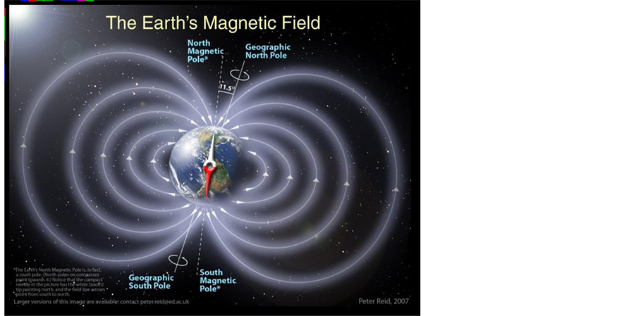
Figure 1. a view of the Earth’s magnetic field.
the air shots have led to substantial improvements in equipment and devices in airborne measuring. The first trial of such shots dates back to the use of a balloon and a receiver conducted on a known deposit in Sweden in 1921. Among the other works done in the following years was the coordination of the flux-gate devices for these studies which were formerly used in maritime studies. The proton precession magnetometer optical pumping (cesium and rubidium vapor) were used in 1951 and 1961, respectively [14] .
Airborne magnetometers are more sensitive than that of similar devices used in land studies. This sensitivity amounts even to 1.1 nano-Tesla in some of modern devices. There are two reasons for taking this sensitivity in consideration. First, the high cost of the plane and having enough space for airborne equipment calls for more advanced devices compared to land-based magnetometers to make most of these shots. Second, considering the shots from height and thus the fact of getting far from the target, it is necessary to use devices with higher sensitivity to obtain more accurate values. In general, the airborne shots are designed to measure overall field and thereupon it is more difficult to interpret vertical or horizontal component of land-based data of the magnetic field. Nowadays, these shots pursue three objectives: Detection, oil exploration and mine exploration. In Canada, by the year 1971, more than half the area of the country was covered by airborne shots. In Iran, aeromagnetic shots were made 1977 under a contract with the Airo at the order of State Geological Organization [15] . Also, during 1972-1978, magnetic shots were conducted over vast regions of the country by some foreign companies under the supervision of Atomic Energy Organization (AEO).
Advantages and Disadvantages of Aeromagnetic Shots
The main advantage of aeromagnetic is its speed which reduces the cost of shots compared to land-based ones. The main part of the cost of airborne shots is associated to assistive devices, because aero magnetometers are not much different from similar devices in terms of price. Surface or near-surface magnetic noise effects often create problems in land-based examinations. In airborne shots, these problems are obviated and thus airborne data are more constant than the others. Airborne shots can be used over vegetated regions, over waters, and hilly lands. For example, in the case of countries like Iran that belongs to regions where there are many communication net- work and exploration problems, airborne shots are of particular advantage [16] .
Among the disadvantages of aero magnetic shots are inaccuracy and costliness in studies which are conducted over low-scale areas. This issue especially holds true concerning the exploration of mineral deposits in the de- tailed and semi detailed stages.
4. The Area under Study
The study area includes 61:100,000 maps of Baghat, Dehsard, Haji Abad, Khabr, Dolat Abad, and Dashtour (Figure 2).
Geophysical Maps of the Area
It is worth mentioning that before beginning interpretation steps, the IGRF correction has to have been conducted on the intensity of the magnetic field. This correction helps obtain input data for interpretation step. IGRF (International Geomagnetic Reference Filed) at each point represents the theoretical values calculated from the universal formula. Each point on the Earth has unique coordinates. Therefore, with coefficients of IGRF univer- sal formula, the overall field intensity, tilt, and deviation angle can be calculated at each point. IGRF coefficients are published by the IAGA Association (International Association of Geomagnetism and Agronomy) at 5-year intervals.
In other words, the IGRF values show a portion of the magnetic field which is of internal origin and have long-term changes. Considering that the purpose of the exploratory magnetometry is to obtain portions of the magnetic field created by subsurface anomalies, IGRF effects can be eliminated from the measurements.
For mapping and data networking, the data obtained from geophysical 1:250,000 map of the Geology Organization are grid-lined with cell dimensions of 275 m and the intensity of the residual magnetic field is obtained (Figure 3).
The maximum and minimum field intensity at this map are 39,900 and 39,420 nano Teslas, respectively. On this map, it is not possible to accurately detect anomalies but it is possible to obtain a notion of how these anomalies are aligned. In fact, to reach the interpretation stage, these data should undergo some corrections and


Figure 2. Location of 1:100,000 maps in the framework of Haji Abad.
processes so that their output map is prepared for interpretation. The general range of anomalies is from the East to the West. Also, in the center of the limit, the anomaly with a weaker intensity is shown.
5. Methodology
Ahmed Salem (2003) combined the two methods analytical signal and Euler's combined method and invented a new combined method to estimate the depth, location and shape of the magnetic and gravity sources [17] .
This method is called AN-EUL (AN-EUL method is an automated method for the interpretation of magnetic and gravity data whose equations are obtained by placing Euler differentiation in analytical signal).
5.1. Producing Analytic Signal Map (AS)
Signal analysis is a method of quantitative interpretation of potential field data. Previous studies demonstrated that the properties of the magnetic body and the magnetized disruption do not affect the analytical signal. This filter of overall magnetic anomaly is independent of the magnetized direction and helps determine the guiding magnetic body. The use of analytical signal for determining the depth of the magnetic body helps reduce the computation complexity and interference effect. Using differentiations indifferent directions, the analytic signal filter eliminates in three directions the regional trend effect which is of the first grade and better shows the magnetic body by eliminating the effect of surface anomalies (noise). Among the problems of this method is the distance of magnetic body from the Earth’s surface in which the less distant it is, the better response we get. The

Figure 3. Residual magnetic map Res TMI.
second problem is the difference between the work of the magnetic body and the surrounding rocks. In which the greater the difference between the analytical signals is clearer map. Horizontal and vertical components in the two-dimensional analytical signal associated to the magnitude of the gradient of the magnetic data are equal to the twist of both horizontal and vertical around all possible deviations. To process magnetic field data, the analytical signal fluctuation is significant in a two-dimensional manner so that we can receive an independent signal from the direction of magnetized source.
The theory of this method is stated based on noise elimination with respect to the differentiation in different directions in that by differentiating in various directions, the effect of regional trend, which is of the first degree, is eliminated and the effect of surface anomalies unrelated to deposits are better eliminated. The magnetic field read by the magnetometer is consisted of the features of magnetic body and intensity of magnetic field in that region which can be separated from each other. If we want to express this in a mathematical formula, we should use Euler and Werner twist.
The maximum amplitude of the analytic signal of the overall anomaly field is independent of magnetized direction and is guiding in determining the magnetic body. Applying this method for determining the depth of the magnetic body decreases complicated calculations and the interference effects.
Using differentiation in different directions, the analytical signal eliminates in three directions the regional trend effect which is of the first type and shows magnetic body better. Based on previous studies, it is confirmed that the properties of the magnetic body and the magnetized direction do not affect the analytical signal. The analytical signal of the overall anomaly field is independent of magnetized direction and is guiding in determining the border of the magnetic body. Analytical signal method is used to determine the edges of anomie and, in some cases, to determine the maximum and minimum depth of the anomaly. The analytical signal for the gravitation gradient is defined as follows:
Equation (2):

And the amplitude of analytical signal is defines as:

To use the above equation in a magnetic method, it suffices to place magnetic field gradients instead of the gravitation gradient, because the location of the maximum analytical signal is right above the edge or corner of anomaly.
This maximum or the maximum analytical signal is located right on the edges of the anomaly. For calculating the analytic signal, first, the horizontal gradient is determined and then the Hilbert transform is used to determine the vertical gradient. The Hilbert transform with no change in the function value creates a change of 90 degrees on the phase spectrum, in other words, the horizontal gradient is transformed into vertical one.
Analytical signal function is a very useful tool in the interpretation of magnetic data. The analytic signal is used to determine the depth of the contact area. Signal analysis is used to determine the location and depth of the magnetic sources. Analytical signal amplitude reaches its maximum value on its body or on the edge depending on the source. Using this feature of the analytical signal, its source and the edges are identified. Regarding the location of spatial windows, the maximum analytical signal amplitude can be obtained in different directions in each window. By connecting the maximum points in each window, a certain limit (border) is obtained for the anomaly. For the points that fall on the borderline, the depth can be estimated using the same window. It should be noted that the operation of analytic signal is done on the polarized data, otherwise, the border detection will be subject to error and the anomaly border is seen with a surface transform.
In this map, the main anomaly border is identified on the east of the determined area. Also, magnetic discon- tinuities are observed in the rest of the high-intensity points which are mainly in the north east, northeast, south- east, center, and north-west.
5.2. Euler Combined Method
Euler combined method is a semi-automated method for estimating the depth, shape and position of the magnetic sources and gravitation. In Euler method, there is no need for transferring to poles and the magnetism left is a disturbing factor.
In this method, the Euler homogeneous differential equation is used. Euler method is applied on profile data (two-dimensional) and network data (three-dimensional).
The function f(x, y, z) is homogeneous of n order if the following equation is for every desired true t coefficient:
Equation (2-0)

In this respect, the function applies in the differential equation:
Equation (3-0)

equation (3-0) is called Euler homogeneous differential equation.
The magnetic field resulting from many simple magnetic sources is as follows:

where a is a constant value and r is the distance from source to measurement point:
Equation (5-0)

With regard to the correlations of equation (2-0) and equation (4-0),
 is a homogeneous function of order-n and applies in the Euler homogeneous equation:
Equation (6-0)

In the equation (6-0), the point (x0, y0, z0) is the location of the source, the point (x, y, z) is the measurement point, and the homogeneous function
 is the magnetic field caused by the source.
The coefficient n is called the structural index which represents the rate of field change with its distance from the source. By knowing n, the general shape of the source can be estimated. Theatrically speaking, the numerical value of the structural index is always greater than zero and negative structural index occurs due to miscalculation or poor quality data. But in some cases, because of noise or errors resulting from numerical miscalculations, a very small negative number may be obtained for the structural index. In the index structure of some of magnetic structures we have:
Generally, the overall calculated field at each point
 can be considered the sum of field resulting from
 source of the regional field
 , in which
 has a constant value:
Equation (7-0)

By placing equation (7-0) in equation (6-0), we have:
Equation (8-0)

This equation must be solved for all grid points or profiles. The parameters B, z0, y0, x0 will be the unknowns in this equation. The solution of the equation (8-0) includes the following steps:
1) We consider a moving window of a given size. We let the number of points on this window be m. The win- dow moves on the grids so as to encompass all measurement points.
2) Due to the fact that there is a certain value of n for all simple sources, a number is assigned to n.
3) Equation (8-0) is solved separately for each window. Since the number of equations (m equations) is higher than the number of unknowns (four unknowns), in each window, the least squares method is used to find the best answer. Then, the window moves and another answer is obtained. In like manner, the windows moves on all grid points and numerous answers obtained.
4) Steps one to two are repeated for various windows and structural indices.
5) That structural index is acceptable for which the answers obtained (depth and location) have a higher concentration [18] .
Thompson (1985) used this method to interpret the profile data and managed to determine the position and shape of the two-dimensional sources. Reid applied this method to the three-dimensional case [19] .
The matrix equation (8-0) is solved using Least Squares method as follows:
Equation (9-0):

And introducing three matrixes A, X, L in equation (9-0)

We have Equation (10-0)

Equation (10-0) is the answers of equation (8-0). Is the Transposed of matrix A [20] . In Euler method, anomalies resulting from the adjacent sources are a separate issue investigated Gregory & Hansen (1996). In Euler method, the horizontal position obtained for the source is selected almost independently of the structural index. Therefore, the horizontal position of the source can be accurately obtained only by selecting a window of a proper size and by ignoring the value of n. However, the wrong choice of structural index can lead to a lot of errors in estimating the depth of the source. It should be noted that the width of the window has a significant im- pact on the accuracy of the estimates of the source [21] .
The weak point of Euler method is the selection of structural index before the application of the method on the data. In addition to the structural index, the selection of parameters such as the maximum depth tolerance, Euler window size, and maximum distance accepted are among the problems arising from this method.
6. Results
In general, one of the features of the analytical signal filtering is to determine the magnetic lineaments and hidden and unhidden faults. In this area, certain lines are determined in the center, North East, South East, and North West of the area which are on magnetic discontinuities with certain trends.Based on the above methodology and by using Oasis software, Figures 4-6 were obtained. In this method, the solving points of Euler equation are extracted in places overlapping with determined magnetic lineaments. Table 1 shows the depth of these points. By using Arc Map 10 software, map of faults extracted were obtained (Figure 7 and Figure 8) and with this software again, incorporation and comparison of existing maps were done and Figures 9-11 were obtained. And finally by using Figure 12 and Figure 13, display of lineaments extracted by remote sensing and aerial geophysics were obtained (Figure 14).
7. Conclusion
According to telemetric investigations conducted either via satellites pictures or geo-magnetic aerial shots, the following results have been obtained. Regarding telemetric studies carried out in ER-mapper, Sharpen 11 is the best filter for display of lineaments.

Figure 4. Map of analytic signal.

Figure 5. Map of magnetic faults and lineaments.

Figure 6. The position of Euler pole.

Figure 7. Map of geomagnetic shots.

Figure 8. Map of faults extracted from all the filters applied.

Figure 9. Map of extracted faults.

Figure 10. Map of faults extracted by geomagnetic data.

Figure 11. F Comparison of the map of magnetically extracted faults with Zag- ros main fault.

Figure 12. Map of divisions of formations and extracted faults.

Figure 13. Display of divisions of main faults and extracted faults.

Figure 14. Display of lineaments extracted by remote sensing and aerial geo- physics.

Table 1. The relationship between the structural index, model type, and the position of calculated depth (2002 Hsu).
Regarding the studies carried out with geomagnetic data, analytical signal is the best filter for specification of lineaments.
The structures extracted by the remote sensing are in accordance with the main Zagros zone in the east-west orientation of the region.
Polymorphism and other ophiolites are in Zagros main thrust zone.
According to the geomagnetic investigations, the main thrust is inclined towards the North East.
The major reason for the change of the region polymorphism is the subsidence of Saudi Arabia zone beneath central Iran. Accordingly, the more we get away from the main thrust, it becomes simpler in structure and the more faults far from the thrust we will have.
The hidden structures of the region are in the east-west direction and are 40 km in depth.
The hidden structures of the region under study are located under the quaternary deposits of Abraham, Dar- bagh, Gilan, Khwaja in a depth of 40 kilometers.
The hidden structures in the North West of the area under study near the town of Aliabad are located in a depth of 4 to 7 km below the ground. In addition, all the extracted faults are recommended for further studies because some of these lineaments and faults are hidden and are located near buildings and, in some cases, under cities. A geophysical and seismic study of the region and recording them in the general map of Iran’s fault is proposed.
References
- Ellis, R.G. and Oldenburg, D.W. (1994) Applied Geophysical Inversion. Geophysical Journal International, 116, 5-11. http://dx.doi.org/10.1111/j.1365-246X.1994.tb02122.x
- Carvalho, J., Cabral, J., Gonçalves, R., Torres, L. and Mendes-Victor, L. (2006) Geophysical Methods Applied to Fault Characterization and Earthquake Potential Assessment in the Lower Tagus Valley, Portugal. Tectonophysics, 418, 277- 297. http://dx.doi.org/10.1016/j.tecto.2006.02.010
- Robinson, D.A., Binley, A., Crook, N., Day-Lewis, F.D., Ferré, T.P.A., Grauch, V.J.S., Slater, L., et al. (2008) Advanc- ing Process-Based Watershed Hydrological Research Using Near-Surface Geophysics: A Vision for, and Review of, Electrical and Magnetic Geophysical Methods. Hydrological Processes, 22, 3604-3635. http://dx.doi.org/10.1002/hyp.6963
- Kneisel, C., Hauck, C., Fortier, R. and Moorman, B. (2008) Advances in Geophysical Methods for Permafrost Investigations. Permafrost and Periglacial Processes, 19, 157-178. http://dx.doi.org/10.1002/ppp.616
- Gibson, P.J., Lyle, P. and George, D.M. (2004) Application of Resistivity and Magnetometry Geophysical Techniques for Near-Surface Investigations in Karsticterranes in Ireland. Journal of Cave and Karst Studies, 66, 35-38.
- Buck, S.C. (2003) Searching for Graves Using Geophysical Technology: Field Tests with Ground Penetrating Radar, Magnetometry, and Electrical Resistivity. Journal of forensic sciences, 48, 5-11.
- Hrouda, F. (1982). Magnetic Anisotropy of Rocks and Its Application in Geology and Geophysics. Geophysical Surveys, 5, 37-82. http://dx.doi.org/10.1007/BF01450244
- Maher, B.A., Thompson, R. and Zhou, L.P. (1994) Spatial and Temporal Reconstructions of Changes in the Asian Palaeomonsoon: A New Mineral Magnetic Approach. Earth and Planetary Science Letters, 125, 461-471. http://dx.doi.org/10.1016/0012-821X(94)90232-1
- Hunt, C.P., Moskowitz, B.M. and Banerjee, S.K. (1995) Magnetic Properties of Rocks and Minerals. Rock Physics & Phase Relations: A Handbook of Physical Constants, Vol. 3. American Geophysical Union, Washington DC, 189-204. http://dx.doi.org/10.1029/RF003p0189 http://wellog.com/RF003p0189.pdf
- McEnroe, S.A., Robinson, P., Langenhorst, F., Frandsen, C., Terry, M.P. and Boffa Ballaran, T. (2007) Magnetization of Exsolution Intergrowths of Hematite and Ilmenite: Mineral Chemistry, Phase Relations, and Magnetic Properties of Hemo-Ilmenite Ores with Micron―to Nanometer―Scale lamellae from Allard Lake, Quebec. Journal of Geophysical Research: Solid Earth (1978-2012), 112. http://onlinelibrary.wiley.com/doi/10.1029/2007JB004973/full http://dx.doi.org/10.1029/2007JB004973
- Opdyke, N.D. and Mejia, V. (2004) Earth’s Magnetic Field. In: Channell, J.E.T., Kent, D.V., Lowrie, W. and Meert, J.G., Eds., Timescales of the Paleomagnetic Field, American Geophysical Union, Washington DC, 315-320.
- Spaldin, N.A. (2010) Magnetic Materials: Fundamentals and Applications. Cambridge University Press, Cambridge. http://dx.doi.org/10.1017/CBO9780511781599
- Luyendyk, A.P.J. (1997) Processing of Airborne Magnetic Data. AGSO Journal of Australian Geology and Geophysics, 17, 31-38.
- Rigoti, A., Padilha, A.L., Chamalaun, F.H. and Trivedi, N.B. (2000) Effects of the Equatorial Electrojet on Aeromagnetic Data Acquisition. Geophysics, 65, 553-558. http://dx.doi.org/10.1190/1.1444750
- Peters, W.S. and Angelis, M.D. (1987) The Radio Hill Ni-Cu Massive Sulphide Deposit: A Geophysical Case History. Exploration Geophysics, 18, 160-166. http://dx.doi.org/10.1071/EG987160
- Bogorodsky, V.V., Bentley, C.R. and Gudmandsen, P.E. (1985) A Brief Survey of the Earth’s Ice Cover and Methods for Its Investigation. In: Bogorodsky, V.V., Eds., Radioglaciology, Springer Netherlands, Amsterdam, 1-15.
- Salem, A. and Ravat, D. (2003) A Combined Analytic Signal and Euler Method (AN-EUL) for Automatic Interpretation of Magnetic Data. Geophysics, 68, 1952-1961. http://dx.doi.org/10.1190/1.1635049
- Gregory, A.W. and Hansen, B.E. (1996) Residual-Based Tests for Cointegration in Models with Regime Shifts. Journal of Econometrics, 70, 99-126. http://dx.doi.org/10.1016/0304-4076(69)41685-7
- Stordal, F., Isaksen, I.S. and Horntveth, K. (1985) A Diabatic Circulation Two-Dimensional Model with Photochemistry: Simulations of Ozone and Long-Lived Tracers with Surface Sources. Journal of Geophysical Research: Atmospheres, 90, 5757-5776.
- Lawson, A.W. (1942) The Vibration of Piezoelectric Plates. Physical Review, 62, 71. http://dx.doi.org/10.1103/PhysRev.62.71
- Ravat, D. (1996) Analysis of the Euler Method and Its Applicability in Environmental Magnetic Investigations. Journal of Environmental and Engineering Geophysics, 1, 229-238.