Optics and Photonics Journal
Vol.06 No.11(2016), Article ID:71970,9 pages
10.4236/opj.2016.611029
Testing Bell’s Theorem with Circular Polarization
Richard A. Hutchin
Optical Physics Company, Simi Valley, CA, USA

Copyright © 2016 by author and Scientific Research Publishing Inc.
This work is licensed under the Creative Commons Attribution International License (CC BY 4.0).
http://creativecommons.org/licenses/by/4.0/


Received: October 17, 2016; Accepted: November 11, 2016; Published: November 14, 2016
ABSTRACT
Bell tests with entangled light have been performed many times in many ways using linear polarizers, but the same tests have never been done with a circular polarizer. Until recently there has never been a true circular polarization beamsplitter―an optical component that separates light directly into left and right handed polarizations. Using a true circular polarization beamsplitter based on birefringent gratings, entangled light has been analyzed with unexpected results.
Keywords:
Entangled Photons, Bell’s Theorem, Circular Polarization, Tests of Quantum Mechanics

1. Introduction
Ever since Bell published his article proving what is now called Bell’s Theorem [1] , there has been a flurry of experiments done to verify various aspects [2] , and entangled light has matured so much that it has even been transitioned into encrypted communications. In all this work, circular polarization beamsplitters were not used for two reasons.
1) There were no real circular polarizers available. The best you could do was put a quarter-wave plate in front of a linear polarizer. What comes out is not circularly polarized but is theoretically supposed to match the transmission if you actually did have a real circular polarizer.
2) Unlike linear polarizers which can be rotated over 180 degrees to give curves that can be used to extract metrics, there are only two circular polarizations―left and right without anything in between. Basically then circular polarizer tests are much less interesting than linear polarizer tests and do not help resolve continuing theoretical questions about Bell tests.
A true circular polarizer was invented about 10 years ago by Prof. Michael Escuti of the University of North Carolina based on a birefringent grating [3] [4] . Unfortunately, this new component has been mostly unknown to optical researchers since it was developed for display purposes and was never called a circular polarizer. The author has been using those gratings to create interferometric trackers for six years [5] , and thus was familiar with its qualities and was able to apply a true circular polarizer to analyze entangled light.
2. Experiment Design
The basic construction of the circular polarization beamsplitter we used here is a birefringent grating of 20 um period which diffracts right circular polarization one direction and left circular polarization the opposite direction with the usual diffraction angle equal to the wavelength divided by the 20 um period. In our case using 806 nm entangled light, this angle is ±0.0403 radians = ±2.3 deg.
The quality we especially value in these gratings is the polarization purity of the transmitted beams. According to ref [3] , the Right and Left circular diffraction orders are >99.8% pure right and left circular polarization, and the very weak zero order has the same polarization state as the input beam. Transmission is typically >95%. This true circular polarization beamsplitter is extremely useful for this QM experiment.
The first test configuration is shown in Figure 1. It was used to verify the two entangled states desired for this experiment.  or
or , which can be selected using a quarter-wave retarder or not. The entangled source was created using the BBO entangled light module from Newlight Photonics. This is a very standard entangled light generator to create a Bell test with linear polarizers. The various hardware elements for this experiment are listed below and photographs of the setup are included in the Appendix.
1) Laser source: Begin with a 50 milliwatt Radius Diode Laser at 403 nm (as calibrated by the manufacturer). Polarization > 100:1 TEM 0.0. Divergence 0.2 × 0.3 millirad. A good commercial laser.
2) BBO down-converter: Standard entangled light module from Newlight Photonics. We added a laser isolator to prevent back reflections, a half-wave plate to rotate the input polarization, a quarter-wave plate to convert linear polarization to circular, and a paired BBO crystal designed to generate down converted photon pairs at +/− 2.8 deg with respect to the incident laser beam.
3) Laser dump: We added a custom deflector to remove the unused 403 nanometer laser beam so as not to interfere with the entangled measurements.
4) Detectors: The detectors are not shown in Figure 1, but they are the very familiar Tau-SPAD detectors with a Hydra-HARP 300 pulse coincidence detector used by many labs to detect coincident photons. They have about 30% QE, and are sometimes used with linear polarizers in front to verify standard entanglement and sometimes with no polarizers when the birefringent grating polarizer above is moved into place.

Figure 1. General layout of the standard test to verify proper photon entanglement.
5) 403 nanometer blocking: Since the laser pump is much brighter than the down- converted light, we used an absorbing plate to absorb any residue 403 nm light prior to reaching the Tau-SPAD detectors while transmitting the 806 nm entangled light. Also we used a narrow band filter of 96% transmission about 4 nm half-width tuned to 806 nm in front of each detector. These additional components reduced the transmission to the detectors to about 90%. However by adding them, any leaked laser light would not show significant counts.
3. Verification of the Entanglement
The first test was to verify a high degree of entanglement with max-to-min = 139:1. We set both polarizers 1 and 2 to nominal vertical and scanned polarizer 2 in 10 degree steps. Our photon count rate was about 10,000 counts per second and coincident counts peaked at 2100 counts per second. In 200 seconds we accumulated up to 400,000 coincident counts per data point. The resulting data is shown in Figure 2. This data showed a total transmission times QE of slightly over 20%. Given our detector QE quoted at 30%, this was reasonable. The theoretical sinusoidal fit matched the data to 1.5× the shot noise limit-an rms noise of 3.2 × 10⁻⁴ on the coincident fraction.
4. Determining the Entangled State
To characterize the relationship between the X1X2 and Y1Y2 states we set linear polarizer 1 to negative 45 deg from nominal vertical (counterclockwise from vertical) and scanned linear polarizer 2 as before from 0-180 (clockwise from vertical). If we were in the  state, then we would expect this response curve to match Figure 3 shifted 45 deg to the left―which would begin with a huge dip over half the cycle (magenta curve in Figure 4). If the Y1Y2 state is not perfectly phased to the X1X2 state, then the modulation would drop a bit, but the general shape of the curve would remain the same. We plotted this curve dropped in modulation to best match the observed data. Clearly it is 180 deg out of phase.
Note: Since the vertical axis is the symmetry axis for this experiment, it got labeled as X. the horizontal axis is labeled as Y.
Conversely, if we were in the  state, then we would expect this response curve to match Figure 3 extended 45 deg to the left―which would begin with a huge rise over half the cycle. Again if the Y1Y2 state is not perfectly phased to the X1X2

Figure 2. Typical entangled photon results from the standard Bell test using linear polarizers in our laboratory. Polarizer 1 was kept stationary and Polarizer 2 was rotated over 360 degrees. Contrast of 139:1 indicated a high level of entanglement for the vertical polarization.

Figure 3. The data where polarizer 1 is rotated 45 deg counterclockwise, match the XX-YY entangled mode and wildly disagree with the XX + YY entangled mode.

Figure 4. The entangled state deduced from the coincidence counts versus angle in Figure 2 and Figure 3 was applied to give an excellent match to the experimental data in Figure 2, where Polarizer 1 and 2 were set to nominal vertical and then Polarizer 2 was scanned over 180 degrees.
state, then the modulation would drop a bit, but the general shape of the curve would remain the same. We plotted this curve dropped in modulation to best match the observed data. Clearly the state  matches the data quite well, while the state
  (magenta curve) curves oppositely. We conclude that we are close to the
  state with a phase shift in the Y1Y2 term to make the modulation drop.
Entangled State Estimation
Given this combined data from Figure 3 and Figure 4 (the blue dots), we then did a precise match of the phase state for both sets of data together and got the following entangled state .
.

With these values we matched the observed data quite well as shown in Figure 4 and Figure 5.
5. QM Predictions for Circular Polarization
Given this measured entangled state, we can rewrite it in terms of right and left circular polarization states, R and L. The quantum state of each of two Type 1 entangled photons is usually written as a superposition of both horizontal (X) and vertical (Y) quantum states as shown in Equation (1), where the subscript 1 or 2 applies to the photon in the first or second path. This is a mathematical way of saying that neither the photon nor nature knows what polarization applies to each photon but whatever they turn out

Figure 5. The entangled state deduced from the coincidence counts versus angle in Figure 2 and Figure 3 was applied to give an excellent match to the experimental data in Figure 3, where Polarizer 1 was set to −45 deg and Polarizer 2 was scanned over 180 degrees.
to be, they are the same.
 (1)
(1)
One can also decompose these linear polarization states into circular polarization states R and L (for right and left circular) using the canonical QM transformation in Equations 2(a) and 2(b) from circular polarization states L and R to linear polarization states X and Y.
 (2a)
(2a)
 (2b)
(2b)
Substituting these Equations (2a) and (2b) into Equation (1), we get Equation 3(a), which reorders into Equation (3b).
 (3a)
(3a)
 (3b)
(3b)
This quantum state predicts that we should observe the two entangled photons with the same handedness 84.8% of the time and with the opposite handedness 15.2% of the time.


6. The Experimental Results
The experiment for circular polarization measurements begins with a verified source of entangled photon pairs, which will then be passed through a circular polarizer to create left and right circular polarized photons. Figure 6 shows a diagram of the experimental setup, and Figure 7 shows a picture.
When we add the circular polarizing birefringent grating in front of the two entangled beams coming from the BBO crystal, we got 4 different beams as shown in Figure 6. Each photon is labeled by its circular polarization (Left or Right) and its entangled beam (1 or 2). These four beams are identified in the drawing. We also remove the rotatable linear polarizers in front of the detectors because the beams now have a fixed and known circular polarization for each beam position. The table layout is shown in Figure 7.
What we found experimentally (Table 1) is that one entangled photon transmits into the left circular polarization path and the other one into the right circular polarization path about 86.3% of the time (opposite handedness). The mean probability of the two photons having the same circular polarization is 13.7%. This is the opposite of QM predictions as shown in Table 1. Due to the high count rates, these data favor the opposite handedness hypothesis by over 300 sigmas compared to the QM predictions.
Example: QM Prediction that R1R2 coincidences are more than L1R2 coincidences is contradicted by (177262 − 24511) = 152751 counts against that hypothesis with a
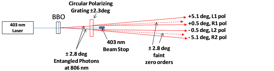
Figure 6. A 403 nm UV laser is sent through a standard BBO Type 1 pair generator from Newlight Photonics. The two entangled beams of 806 nm light were passed through a circularly polarizing grating of 20 um period from Imagin Optix. The two weak zero orders pass through undeflected, while left circular light is deflected left and right circular light is deflected right. Standard Tau-SPAD detectors connected to a Pico-HARP 300 are used to find coincident counts.

Table 1. Data taken with the circular polarization experiment for entangled photons showing that coincidences happen in the reverse handedness predicted by quantum mechanics.
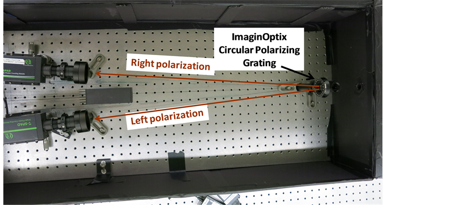
Figure 7. Bell test experiment for circular polarization. The entangled photon generator is behind the black wall on the right.
standard deviation = sqrt(177262 + 24511) = 449 counts. The result is 340 sigmas against the QM prediction. There are four possible tests such as this one―all showing strong statistics against the QM predictions.
7. Conclusion
An experiment was setup using circular polarization to test QM predictions for entangled photons. While the entangled setup performed normally using linear polarizers, it performed opposite to QM predictions with circular polarization with over 300 sigmas of statistical significance. Since circular polarization tests have never been reported for Bell tests before, these results suggest that other entangled facilities should repeat these tests to see if they find the same discrepancy. If other tests confirm these results, then more experiments can be done to understand and model these effects better.
Acknowledgements
The author would like to acknowledge many useful discussions with Dr. Reinhard Erdman, who is a strong supporter of quantum mechanics and skillfully debated the standard QM theory.
Also, the setup and the data acquisition of this experiment were handled excellently and patiently by Mr. Chris Warren.
Cite this paper
Hutchin, R.A. (2016) Testing Bell’s Theorem with Circular Polarization. Optics and Photonics Journal, 6, 289-297. http://dx.doi.org/10.4236/opj.2016.611029
References
- 1. Bell, S. (1964) On the Einstein Podolsky Rosen Paradox. Physics, 1, 195-200.
- 2. Bruner, N., et al. (2014) Bell Nonlocality. Reviews of Modern Physics, 86, 419.
http://dx.doi.org/10.1103/RevModPhys.86.419 - 3. Komanduri, R.K., Jones, W.M., Oh, C. and Escuti, M.J. (2007) Polarization-Independent Modulation for Projection Displays Using Small-Period LC Polarization Gratings. Journal of the Society for Information Display, 15, 589-594.
- 4. Oh, C. and Escuti, M.J. (2008) Achromatic Diffraction from Polarization Gratings with High Efficiency. Optics Letters, 33, 2287-2289.
http://dx.doi.org/10.1364/OL.33.002287 - 5. Hutchin, R.A. (2016) Two Axis Interferometric Tracking Device and Method. US Patent 9297880.