Optics and Photonics Journal
Vol.4 No.1(2014), Article ID:42229,7 pages DOI:10.4236/opj.2014.41001
Vortex Field Propagation in a Hexagonal Multicore Fiber Array
Department of Electrical Engineering and Computer Science, University of Wisconsin-Milwaukee, Milwaukee, USA
Email: mmushref@yahoo.co.uk, mmushref@gmail.com
Received November 22, 2013; revised December 17, 2013; accepted January 5, 2014
ABSTRACT
The propagation of an optical vortex in a hexagonally arranged single mode multicore fiber structure is investigated for possible generation of additional vortices and their spread dynamics. Fields are separated into a slowly varying paraxial envelope and a rapidly changing exponential component. Solutions are derived from the paraxial inhomogeneous Schrodinger equation in two dimensions along with the index of refraction of the proposed structure. Numerical analyses are based on the beam propagation method and transparent boundary conditions in matrix form with different parameters to represent the intensity and phase of all derived fields. Vortices are numerically identified by their points of zero intensity and their phase change or polarity. The optical interferogram with a plane wave reference is also employed to distinguish the dislocation points in the transverse directions of the propagating fields.
Keywords:Optical Vortex; Beam Propagation Method; Transparent Boundary Conditions; Multicore Fibers; Optical Interferogram
1. Introduction
The propagation of light and its waveguiding properties in periodic lattices or multicore fibers is one of the important fields of study in photonics. Optical vortices travelling in such structures form a very rich area of research due to their intensity and phase features. The significant implication is their possible attractive applications in optical switching, modulation and sensing [1,2]. There are several theoretical and experimental published studies in the literature that examined the propagation of optical vortices and their overall behavior. Though, previous investigations did not verify possible relations between newly generated vortices and the propagation distance with the effects of different parameters such as structure size and number of cores.
Dispersion and size of guided beams are numerically determined for an optical vortex soliton in a graded index waveguide [3]. The propagation of a stationary pulse in circularly arranged coupled cores is also numerically examined [4]. The fundamental and vortex solitons in a two-dimensional optical lattice are then considered for the effects of weak and strong localizations on vortex stability [5]. An asymmetric vortex soliton is shown to exist in symmetric periodic lattices by using the energy-balanced relations [6]. In addition, discrete vortex solitons in optically induced photonic lattices are observed experimentally, and their stabilization is verified in a self focusing nonlinear medium [7]. In another experimental investigation, Gaussian and vortex beams and vortex lattice interactions are examined [8]. Moreover, optical vortices are explored to demonstrate stability in two-dimensional photonic lattices with Kerr nonlinearity [9]. Also, observation of topologically stable multivortex solitons in hexagonal photonic lattices is achieved through self trapping of truncated two-dimensional Bloch waves [10]. In similar photonic lattices, stable double charge vortex solitons created in self focusing nonlinear media are observed by experiments [11]. Also, in hexagonal photonic lattices, single charge vortices are found to exhibit dynamical instabilities and thus their breakup occurs at short propagation distances compared to double charge vortices [12].
2. Formulation and Method
The relation between the generated optical vortices in a multicore fiber and the propagation distance is yet to be explored. In this paper, the propagation of an optical vortex in a multicore fiber is theoretically and numerically investigated. All cores are assumed single mode and identical such that they are of equal radius in a hexagonal arrangement with equal distances from each other and with the same index of refraction in a step profile. An example for the proposed structure is shown in Figure 1 for 19 cores in a normalized rectangular coordinates as X = x/w0 and Y = y/w0 with a normalized radius of each core as R = r/w0 and a normalized distance between cores as D = d/w0 where w0 is the beam width and r and d are in μm. The index of refraction of each core is assumed very close to that of free space with a difference of  approximately where n0 = 1.0 for free space. Beam propagation method (BPM) with transparent boundary conditions (TBC) are employed to solve for the propagating optical vortex beam in the proposed multicore fiber [13-15]. Different parameters are also considered in the solutions such as number of cores, core size and their distances from each other.
The solutions start from the source-free Maxwell’s equations to find the Helmholtz scalar wave equation for the field ψ(x, y, z) in the rectangular coordinate system as  where n(x, y) is the refractive index of the medium. In beam propagation method, backward waves are ignored and the fields are separated as a paraxial slowly varying envelope f(x, y, z) multiplied by a rapidly varying exponential part in the form
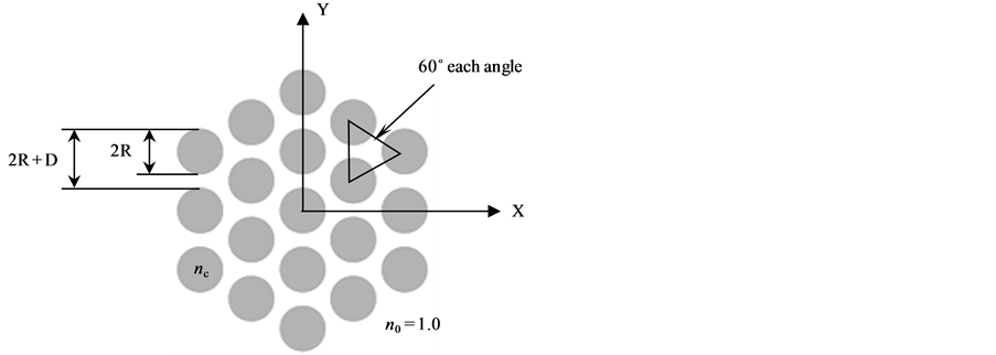
Figure 1. Schematic transverse section of the proposed structure with 19 cores in hexagonal arrangement.
[16]:
![]() (1)
(1)
where n0 and k0 are the free space index of refraction and wavenumber respectively.
By substituting Equation (1) in the Helmholtz scalar wave equation, the propagation of the optical field can be described by the inhomogeneous normalized Schrodinger equation in the form [15]:
 (2)
(2)
where,  ,Φ(X, Y, Z) is the normalized paraxial slowly varying field envelope, n (X,Y) is the structure refractive index, Z = z/z0, z0 = π w02/λ and λ is the wavelength.
3. Numerical Analyses
Equation (2) is numerically solved for the field Φ(X, Y, Z) using finite difference (FD) and split-step techniques by employing the calculation steps of X = Xm = mΔX, Y = Yp = pΔY and Z = Zq = qΔZ [16]. Calculation steps are assumed as m = 1, 2, 3, ···, M, p = 1, 2, 3, ···, P and q = 1, 2, 3, ···, Q, where M and P are the transverse field resolution with an assumption of M = P = N. Also, Q is the number of longitudinal steps in Z which is the direction of field propagation along the optical waveguide. Thus, Equation (2) can be split to generate two equations in the form:
 (3a)
(3a)
 (3b)
(3b)
where  is the influence of the fiber lattice material, F* is a numerical intermediate value of the normalized field, A = 1 − α, B = 1 + α, C = α/2, α = jΔZ/4Δ2 and ΔX = ΔY = Δ.
In order to numerically solve Equations (3a) and (3b), they are transformed to matrix form as:
 (4a)
(4a)
 (4b)
(4b)
where F and G are the right hand expressions in Equations (3a) and (3b) respectively and L is an N × N tridiagonal matrix given by:
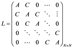 (5)
(5)
The transverse distribution of the initial field is assumed to be Φ1 for q = 1 and it is used in Equation (4a) at the beginning of the solution. Once Φ*1 is calculated, it is then used in Equation (4b) to solve for Φ2 which is the field in the next longitudinal step at q = 2. This process is repeated for any required distance in the normalized longitudinal direction.
The initial normalized optical vortex at Z = 0 can be expressed as a Laguerre-Gaussian mode of the first order given by [17]:
 (6)
(6)
where  is the vortex optical field, j =
 , ρ2 = X2 + Y2 and φ = tan−1 (Y/X).
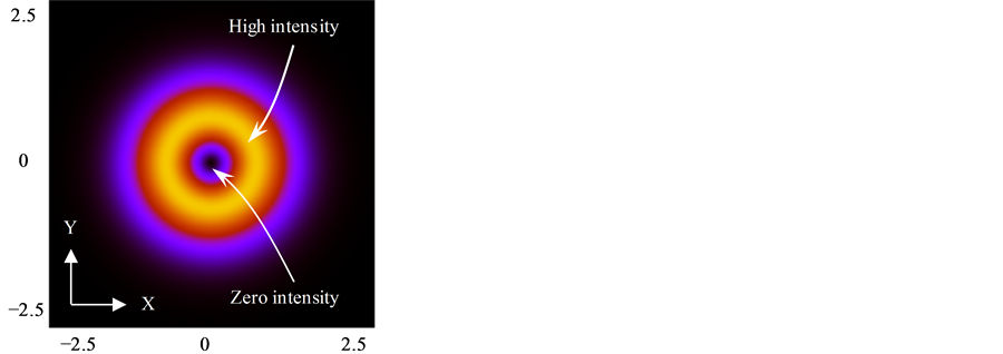
Figure 2 illustrates the initial optical vortex used in this paper which is numerically generated for N = 500, Δ = 0.01, w0 = 5 μm and λ =1.5 μm with y = x and x = Xw0 = NΔw0 = 25.0 μm. The field intensity is shown in Figure 2(a) with the point of zero intensity at the origin and Figure 2(b) shows the phase change from –π to π. Figure 2(c) is the interferogram with a plane wave reference that shows the point of dislocation with a vortex topological charge or polarity of +1 at the origin.
4. Results and Discussions
All analyses and simulations are performed for nc = 1.005, beam width of w0 = 5.0 μm and wavelength of λ = 1.5 μm with  52.36 μm. Single mode cores are assumed with a V number as
where  is the numerical aperture.
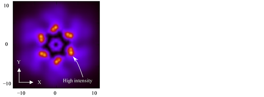
The propagated optical vortex field at Z = 8 (z = Zz0 = 418.88 μm) is shown in Figure 3 for 61 cores with R = 0.4 (r = Rw0 = 2.0 μm), D = 0.2 (d = Dw0 = 1.0 μm), a resolution of N = 1000 and calculation steps of Δ = 0.09 and ΔZ = 0.01. Figure 3(a) is a zoomed in image of the field intensity that illustrates the spots of light in some cores. Since the cores are very close to each other at a constant distance, the field is coupled between them as it propagates. The phase of the field with charges of +1 or −1 of newly generated vortices is shown as a zoomed in image in Figure 3(b) where they demonstrate a phase change from –π to π. The total charge or polarity of vortices should be conserved to +1 which is the charge of the initial transmitted vortex field. Topological charge should be always conserved when new optical vortices are formed and then annihilated in pairs with opposing
 (a)
(a)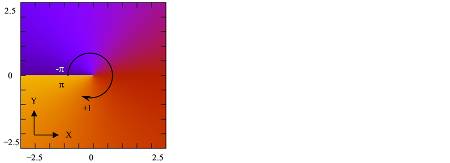 (b)
(b)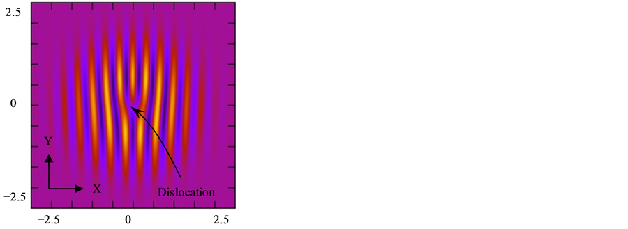 (c)
(c)
Figure 2. Intensity (a), phase (b) and interferogram with a plane wave reference (c) of an optical vortex for N = 500, Δ = 0.01, w0 = 5 μm and λ = 1.5 μm.
charges [18]. In this case, conservation is confirmed as 7 * (+1) + 6 * (−1) = +1 where there are 7 vortices with +1 charge and 6 vortices with −1 charge. Figure 3(c) is the zoomed in image of the interferogram with a plane wave reference at an angle of π/4 with respect to the X axis which also displays the dislocation points of vortices at comparable locations to that shown in Figure 3(b).
 (a)
(a)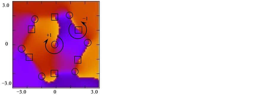 (b)
(b)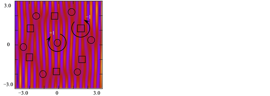 (c)
(c)
Figure 3. Intensity (a), phase (b) and interferogram with a plane wave reference (c) of an optical vortex for N = 1000, Δ = 0.09, Z = 8.0, w0 = 5 μm and λ =1.5 μm. ¨ = −1 charge and ¡ = +1 charge.
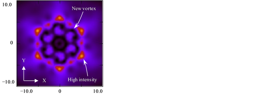
Moreover, Figure 4 shows the propagated optical vortex field at Z = 11 for 127 cores with R = 0.4, D = 0.2, a resolution of N = 1000 and calculation steps of Δ = 0.04 and ΔZ = 0.01. Figure 4(a) is a zoomed in image from −10.0 to 10.0 of the field intensity with the spots of light coupled and spread in more cores compared to the case
 (a)
(a)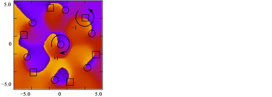 (b)
(b)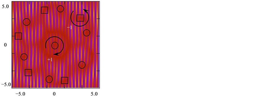 (c)
(c)
Figure 4. Intensity (a), phase (b) and interferogram with a plane wave reference (c) of an optical vortex for N = 1000, Δ = 0.04, Z = 11.0, w0 = 5 μm and λ = 1.5 μm. ¨ = −1 charge and ¡ = +1 charge.
in Figure 3(a). The phase of the field from –π to π is shown as a zoomed in image in Figure 4(b) with 6 new pairs of vortices around the first vortex at the origin which demonstrate the conservation of charge. Also, Figure 4(c) shows the zoomed in image of the interferogram with a plane wave reference at an angle of π/4 with respect to the X axis that shows the points of dislocations for each created vortex.
The approach discussed in Figures 3 and 4 is employed to investigate the generation of new vortices with respect to Z when the number of cores, R or D parameters are varied. Results are listed in Table 1 for Z from 0.0 to 20.0 when the number of cores is 37, 61, 91 and 127 respectively and visualized in Figure 5 for R = 0.4 and D = 0.2 for the same number of cores. Polarities of new vortices are also recorded in Table 1 which clearly demonstrate and confirm the conservation of charge. The curves shown in Figure 5 have meaning only at the data points in Table 1 at integer values for the same parameters. As exposed, the generation of new vortices is very dynamic and highly varied with respect to Z and the number of cores. More vortices are created as the number of cores increases and the beam propagates at farther distances. New vortices start to appear at shorter propagation distance but more new vortices are produced when the

Table 1 . Generated vortices for different number of cores for R = 0.4 and D = 0.2 (polarities are shown between parentheses).
number of cores is higher. However, new vortices could not exist continually and may possibly vanish with other new vortices generated at different locations.
As in Table 1, the longitudinal distance at Z = 8.0 shows differences in the number of new vortices as the number of cores is varied. Core radius may also affect the number of new generated vortices as listed in Table 2 and visualized in Figure 6 for R = 0.2, 0.3 and 0.4, Z = 8.0 and D = 0.2 for the same number of cores. The generation of new vortices is very sensitive to the core radius when there are more cores such as the sharp change from 1 vortex to 11 vortices and then to 1 vortex for 127 cores.
In addition, variation of the distance between cores could show some changes in the number of new vortices as listed in Table 3 and visualized in Figure 7 for D =
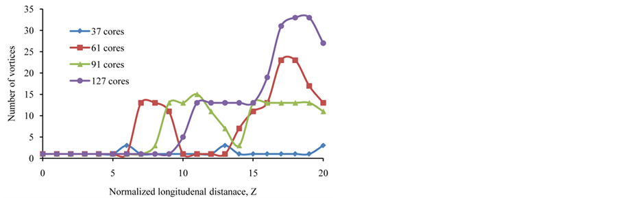
Figure 5. Created vortices with respect to Z for different cores for R = 0.4 and D = 0.2.
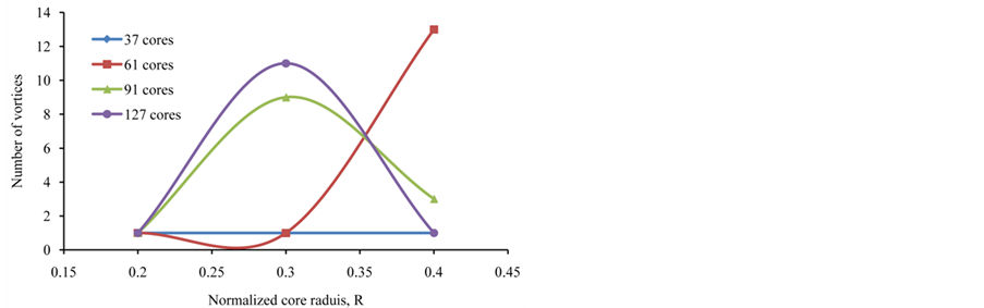
Figure 6. Created vortices with respect to R for different cores for Z = 8.0 and D = 0.2.
Table 2. Generated vortices with core radius R for different number of cores for Z = 8.0 and D = 0.2 (polarities are shown between parentheses).
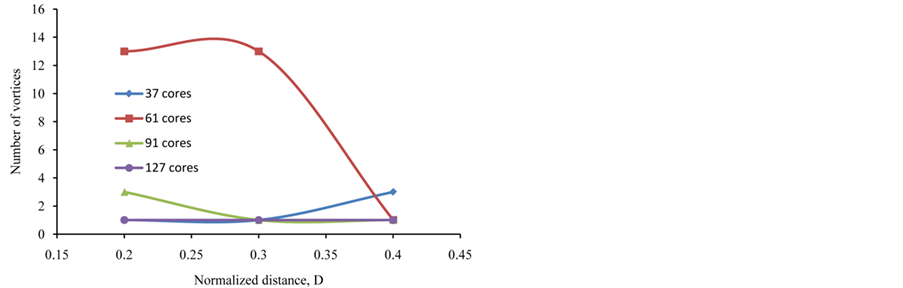
Figure 7. Created vortices with respect to D for different cores for Z = 8.0 and R = 0.4.
Table 3. Generated vortices with distance D for different number of cores for Z = 8.0 and R = 0.4 (polarities are shown between parentheses).
0.2, 0.3 and 0.4, R = 0.4 and Z = 8.0. This parameter may have an increasing effect such as the change of the number of vortices from 1 to 3 in a 37 cores array. Also, it could have a decreasing effect such as the change from 13 to 1 in a 61 cores array or from 3 to 1 in a 91 cores array.
5. Conclusion
Theoretical analyses are presented for the propagation of an optical vortex field in a single mode multicore fiber array. The derivations employed beam propagation method and transparent boundary conditions to obtain the numerical solutions. Investigations explained the highly dynamical nature of the propagating vortex in the proposed structure. Different parameters were examined such as the number of cores and the size of the structure that could have an effect on the creation of new vortices. It is found that vortices are very responsive to variations of the array parameters either by increasing or by decreasing the number of vortex pairs given that the topological charge is conserved.
REFERENCES
- D. N. Christodoulides, F. Lederer and Y. Silberberg, “Discretizing Light Behavious in Linear and Nonlinear Waveguide Lattices,” Nature, Vol. 424, No. 6950, 2003, pp. 817-823. http://dx.doi.org/10.1038/nature01936
- J. Demas, M. D. W. Grogan, T. Alkeskjold and S. Ramachandran, “Sensing with Optical Vortices in PhotonicCrystal Fibers,” Optics Letters, Vol. 37, No. 18, 2012, pp. 3768-3770. http://dx.doi.org/10.1364/OL.37.003768
- C. Law, X. Zhang and G. Swartzlander Jr., “Waveguiding Properties of Optical Vortex Solitons,” Optics Letters, Vol. 25, No. 1, 2000, pp. 55-57. http://dx.doi.org/10.1364/OL.25.000055
- A. Buryak and N. Akhmediev, “Stationary Pulse Propagation in N-Core Nonlinear Fiber Arrays,” IEEE Journal of Quantum Electronics, Vol. 31, No. 4, 1995, pp. 682- 688. http://dx.doi.org/10.1109/3.371943
- J. K. Yang and Z. H. Musslimani, “Fundamental and Vortex Solitons in a Two-Dimensional Optical Lattice,” Optics Letters, Vol. 28, No. 21, 2003, pp. 2094-2096. http://dx.doi.org/10.1364/OL.28.002094
- T. J. Alexander, A. A. Sukhorukov and Y. S. Kivshar, “Asymmetric Vortex Solitons in Nonlinear Periodic Lattices,” Physical Review Letters, Vol. 93, No. 6, 2004, pp. 63901-63905. http://dx.doi.org/10.1103/PhysRevLett.93.063901
- D. N. Neshev, T. J. Alexander, E. A. Ostrovskaya, Y. S. Kivshar, H. Martin, I. Makasyuk and Z. G. Chen, “Observation of Discrete Vortex Solitons in Optically Induced Photonic Lattices,” Physical Review Letters, Vol. 92, No. 12, 2004, pp. 123903-123906. http://dx.doi.org/10.1103/PhysRevLett.92.123903
- Z. G. Chen, H. Martin and A. Bezryadina, “Experiments on Gaussian Beams and Vortices in Optically Induced Photonic Lattices,” Journal of the Optical Society of America B, Vol. 22, No. 7, 2005, pp. 1395-1405. http://dx.doi.org/10.1364/JOSAB.22.001395
- M. I. Rodas-Verde and H. Michinel, “Dynamics of Vector Solitons and Vortices in Two-Dimensional Photonic Lattices,” Optics Letters, Vol. 31, No. 5, 2006, pp. 607-609. http://dx.doi.org/10.1364/OL.31.000607
- B. Terhalle, T. Richter, A. S. Desyatnikov, D. N. Neshev, W. Krolikowski, F. Kaiser, C. Denz and Y. S. Kivshar, “Observation of Multivortex Solitons in Photonic Lattices,” Physical Review Letters, Vol. 101, No. 1, 2008, pp. 13903-13906. http://dx.doi.org/10.1103/PhysRevLett.101.013903
- B. Terhalle, T. Richter, K. J. H. Law, D. Gories, P. Rose, T. J. Alexander, P. G. Kerekidis, A. S. Desyatnikov, W. Krolikowski, F. Kaiser, C. Denz and Y. S. Kivshar, “Observation of Double-Charge Discrete Vortex Solitons in Hexagonal Photonic Lattices,” Physical Review A, Vol. 79, No. 4, 2009, pp. 43821-43829. http://dx.doi.org/10.1103/PhysRevA.79.043821
- K. J. H. Law and P. G. Kevrekidis, “Stable Higher-Charge Discrete Vortices in Hexagonal Optical Lattices,” Physical Review A, Vol. 79, No. 2, 2009, pp. 25801-25805. http://dx.doi.org/10.1103/PhysRevA.79.025801
- C.-S. Hsiao, L. Wang and Y. J. Chiang, “An Algorithm for Beam Propagation Method in Matrix Form,” IEEE Journal of Quantum Electronics, Vol. 46, No. 3, 2010, pp. 332-339. http://dx.doi.org/10.1109/JQE.2009.2029066
- S. A. Shakir, R. A. Motes and R. W. Berdine, “Efficient Scalar Beam Propagation Method,” IEEE Journal of Quantum Electronics, Vol. 47, No. 4, 2011, pp. 486-491. http://dx.doi.org/10.1109/JQE.2010.2091395
- D. Jimenez and F. Perez-Murano, “Improved Boundary Conditions for the Beam Propagation Method,” IEEE Photonics Technology Letters, Vol. 11, No. 8, 1999, pp. 1000-1002. http://dx.doi.org/10.1109/68.775326
- K. Okamoto, “Fundamentals of Optical Waveguides,” Elsevier Inc., Maryland Heights, 2006.
- B. Saleh and M. Teich, “Fundamentals of Photonics,” John Wiley & Sons, Inc., Hoboken, 2007.
- G. P. Karman, M. W. Beijersbergen, A. van Duijl and J. P. Woerdman, “Creation and Annihilation of Phase Singularities in a Focal Field,” Optics Letters, Vol. 22, No. 19, 1997, pp. 1503-1505. http://dx.doi.org/10.1364/OL.22.001503