Optics and Photonics Journal
Vol. 3 No. 5 (2013) , Article ID: 36242 , 6 pages DOI:10.4236/opj.2013.35047
Application of the Sampling and Replication Operators to Describe Mode-Locked Radiation
Max Born Institute for Nonlinear Optics and Short Pulse Spectroscopy, Berlin, Germany
Email: agitin@mbi-berlin.de
Copyright © 2013 Andrey V. Gitin. This is an open access article distributed under the Creative Commons Attribution License, which permits unrestricted use, distribution, and reproduction in any medium, provided the original work is properly cited.
Received May 9, 2013; revised June 12, 2013; accepted July 8, 2013
Keywords: Mode-Locked Lasers; Sampling Operator; Replication Operator
ABSTRACT
Sampling and replication operators are used for a description of the mode-locking radiation. Such description allows to take into account the influence of the shape of the gain curve of the active medium of the mode-locking laser on the form of the pulses generated by it.
1. Introduction
According to the uncertainty principle, the shorter the pulse duration, the wider the bandwidth of its spectrum. The cycle period of the central frequency of the spectrum is the natural limit of the pulse duration. The pulse which duration is near this natural limit, is called an ultra-short pulse (USP) [1-3].
The main method used to generate USPs is the modelocking technique [4-10]. Traditionally, more than forty years, the formation of mode-locking radiation is described in the form proposed by Yariv [10]. However, in recent papers [11-13] this process is described by using mathematical properties of the “Dirac comb”. Note that, in contrast to traditional one, this description allows to take into account the influence of the shape of the gain curve of the active medium on the form of the generated USPs. Therefore, it makes sense to consider this approach in more detail, using canonical mathematical forms. These canonical forms are sampling and replication operators [14,15].
2. Fourier Transformations and Their Properties
Let us define a forward Fourier transformation [14-16] as
 , (1a)
and an inverse Fourier transformation as
 . (1b)
For example, . Hereafter, a bar on top of the symbol indicates the corresponding function in the frequency domain.
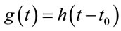
Translation property For any real number w0, if , then
 . (2)
. (2)
Modulation property For any real number t0, if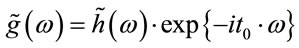 , then
 . (3)
. (3)
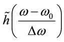
Scaling property For a non-zero real number Dw (the so-called “width parameter”), if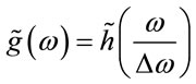 , then
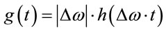 . (4)
. (4)
Two functions g(t) and , each of which is the Fourier transform of the other, are a so-called Fourier transform pair. Usually the functions g(t) and
  are different. For example, if
 (5a)
(5a)
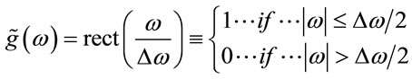
is a rect-function (top-hat function), then
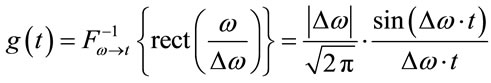 . (5b)
In contrast, a Gaussian function
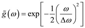 (6a)
(6a)
and its Fourier transform
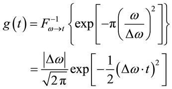 (6a)
(6a)
both are bell-shaped functions.
Convolution theorem , (7)
, (7)
where  is a convolution, i.e., Ä denotes the convolution operator.
Dirac delta function The Dirac delta function can be abstractly defined by two conditions
1) d(t) = 0 for t ¹ 0;
2) .
.
This function has the “sifting property”
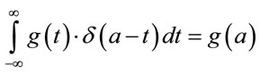 . (8)
. (8)
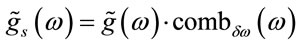
Dirac comb (“sampling function”)
The Dirac comb is a periodic function constructed from Dirac delta functions [14,15]. In the frequencydomain, the Dirac comb is defined as (Figure 1(a)).
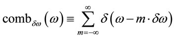 , (9a)
and in the time-domain, it is defined as (Figure 1(d))
 . (9b)
The Fourier transformation of a Dirac comb in the frequency-domain is proportional to a Dirac comb in the time-domain (Figures 1(a), (d)).
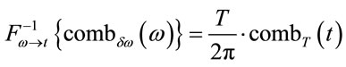 , (10)
where the time-domain “tooth spacing” T and the frequency-domain “tooth spacing” dw are related by the expression.
 . (11)
Two operators are closely related with the Dirac combs and the convolution theorem: the sampling operator and the replication operator [14,15].
Sampling operator If we take a continuous function  (Figure 1 (b)) and multiply it by a Dirac comb, combdw (w) (Figure 1 (a)), we obtain a sampled version
  of this function, i.e., a series of spikes with amplitudes that are equal to the continuous function at a set of discrete points, m×dw (Figure 1 (c)).
 . (12)
Remarks:
Theoretically, the sampled result is a string of delta functions, each of which has an area that equals the value of the continuous signal at the corresponding discrete point, where the digitized points are of the form m×dw. Practically, we can view this result as a series of spikes with amplitudes that are equal to the continuous signal at the discrete points m×dw. This view corresponds to viewing the Dirac comb as having teeth, each with unit amplitude and separated by dw, even though this is formally incorrect [15].
Replication operator The Fourier transformation of a Dirac comb in the frequency-domain (Figure 1(b)) is a Dirac comb in the time-domain (Figure 1 (e)), as shown in Equation (10), and multiplication in the frequency domain is equivalent to convolution in the time domain, as shown in Equation (7). Thus, in the time domain, Equation (12) takes the form
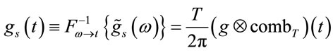 . (13)
If a continuous function g(t) is 0 everywhere except for 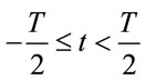 (Figure 1(e)), then its convolution in the time domain with a Dirac comb, combT(t) (Figure 1(d)), replicates g(t) and gives a periodic function gs(t) with periodicity T (Figure 1(f)).
3. Amplifier for USPs
A USP can be described by a complex amplitude U(t) or by its complex spectrum , which presents the USP as a set of monochromatic waves with different angular frequencies w. Both descriptions are complete and also equivalent, because one can be derived from the other by Fourier transformation.
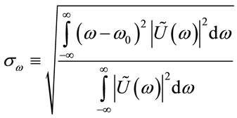
According to Parseval’s theorem
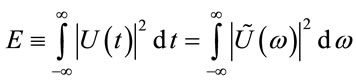 . (14)
if a the distribution of a function u(t) resembles a bell curve (Figure 1(a)) with a temporal peak at
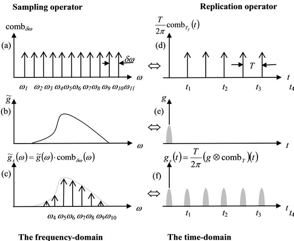
Figure 1. An illustration of the operation of the sampling operator in the frequency domain (a, b, c) and of the replication operator in the time domain (d, e, f). (a) The Dirac delta comb. (b) The function to be sampled. (c) The result of multiplying parts (a) and (b) together, resulting in a sampled function in the frequency domain. The right column shows the corresponding time-domain functions. The symbol Û denotes Fourier transformation.
 , (15a)
and a standard deviation (duration) of
 , (15b)
then its Fourier transform also resembles a bell curve (Figure 1(b)) with a central frequency of
 (16a)
(16a)
and a standard deviation (that is, the bandwidth of the spectrum) of
 . (16b)
In general, the trade-off between these standard deviations can be formalized in the form of an uncertainty principle [17]:
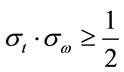 . (17)
The uncertainty inequality given by (17) is the limiting case of the general inequality obeyed by the product of the variances of Fourier transform pairs. The equality
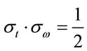 (18)
(18)
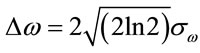
holds only if U(t) has the form of a Gaussian function. Note that the convention is to define the duration of a laser pulse, Dt, and its spectral width, Dw, as the “full width at half maximum” (FWHM) of the functions
 and
and , respectively [18]. When the considered functions are the Gaussian distributions, the relationships between the FWHM and the standard deviations (15b) and (16b) are
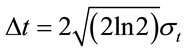 , (19a)
 . (19b)
In these terms the “uncertainty relation” (17) takes the form [3]
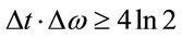 . (20)
An amplifier is an active filter with a frequency characteristic  [1,3] such that
 , (21)
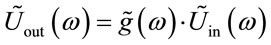
A quantum amplifier transforms an input pulse  into an output pulse
 . In this case the role of the frequency characteristic is played by the gain curve of the active medium that the amplifier is constructed from. As a rule, the gain curve has a maximum M (M > 1) at a frequency w0 and a width Dw:
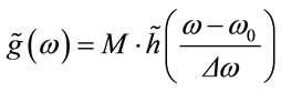 , (22)
where  is the gain curve normalized by the condition
 .
.
In a quantum amplifier, the bandwidth of the spectrum of the input pulse is limited by the bandwidth Dw of the gain curve of the active medium  as may be inferred from Equation (21). Note that any active medium corresponds to the perfect input USP in which a complex amplitude UPerfect(t) = Uin(t) is proportional to the inverse Fourier transformation of the normalized gain curve of the active medium
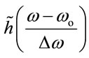 . Thus, taking into account the translation (2) and scaling (4) properties, we have
 . (23)
According to the uncertainty principle (20), the shorter the pulse is, the broader its spectrum must be (and vice versa). The duration of the perfect USP is the minimum duration for the pulse, which is acceptable for amplification in the active medium that has a gain curve of bandwidth Dw. Thus, for amplification of extremely short laser pulses, the gain curve of the active medium must have the widest possible bandwidth Dw.
4. Mode-Locked USP Generator
Note that an input pulse  to a quantum amplifier is often called its “seed pulse”
 . Before amplifying the seed pulse, it is necessary to generate it. An amplifier can be converted into a generator, provided a positive feedback loop is entered [19]. Noise, produced by the amplifier, travels around the loop through a filter and is re-amplified. The spectrum of a generated seed pulse
  is related with the frequency characteristics of the amplifier
  and the feedback filter
  by the equation
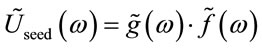 . (24)
In quantum optics, the feedback is provided by a resonant cavity around the gain material. The simplest resonant cavity consists of only two plane mirrors (a high reflector and an output coupler) facing each other, surrounding the gain medium (this arrangement is known as a Fabry-Perot cavity). Since light is a wave, when bouncing between the mirrors of the cavity, the light will constructively and destructively interfere with itself, leading to the formation of standing waves or modes between the mirrors (Figure 2). The condition for constructive interference is
ml = 2L, (25)
where L is the cavity length and m is a large integer representing the number of modes in the standing wave pattern [10].
The condition (25) for the existence of the m-th mode of the laser cavity corresponds to the condition for its frequency
 , (26)
where T º 2L/c is the resonator (cavity) round-trip time. Hence, the frequencies of the adjacent modes are separated by the intermode frequency spacing:
 . (27)
Thus, the complex amplitude of the m-th mode of the resonator is [10]
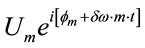 , (28)
where Um is the amplitude, and jm is the phase.
If the width Dw of the gain curve of the active laser
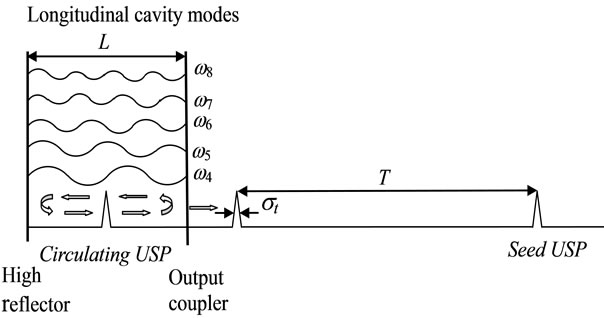
Figure 2. When all the longitudinal modes of the laser cavity oscillate in phase, the laser generates USPs.
medium is much broader than the intermode frequency spacing dw, then the radiation of the laser consists of  modes generated at once. The resulting radiation of the laser is a sum of the modes. The summation of the complex amplitudes of the individual modes depends on their phases. If the phases jm change randomly in time, the sum produces only a rather noisy signal. However, if the phase jm of all the modes are “locked” [10], i.e.,
 , (29)
then the sum forms a pulse localized in a small time interval, i.e., a USP. Note that the condition (29) can be written as the product of the intermode frequency spacing and any value t0:
 . (30)
The value t0 can be interpreted as the time of the peak of the pulse. Thus, for the case of phase-locking, the complex amplitude of the m-th mode Equation (28) can be rewritten in the form
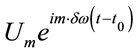 . (31)
Thus, assuming that all the amplitudes of the oscillating modes are equal
Um = const for all modes, m ∈ N, (32)
the frequency characteristic of the resonant cavity  can be written using the translation property (2) and the definition of the Dirac comb (9a) as (Figure 3(a))
 . (33)
Let us suppose that the influence of the dispersion of the gain material on the intermode frequency spacing dw can be neglected. Then, according to Equation (24), the spectrum of the radiation  from a mode-locked generator can be written as a sampled version (Figure 3(c)) of the continuous gain curve of the active medium (Figure 3(b)) in the frequency-domain
 . (34)
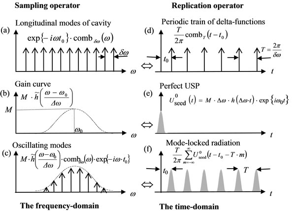
Figure 3. Mode-locked radiation in the frequency-domain (a, b, and c) and in the time-domain (d, e, and f).
By using the convolution theorem and the translation and modulation properties of the Fourier transformation, we obtain an expression for the complex amplitude of the mode-locked radiation in the time domain, which consists of the perfect pulse replicated infinitely by the replication operator. It is given by
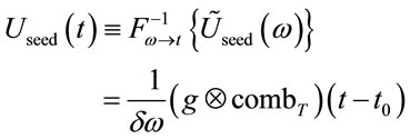 (35)
(35)
Since the round-trip time T is much greater than the duration Dt of the perfect USP, the pulses are well separated from each other. In this case, using the “sifting property” of the Dirac delta function (8) and the definition of the perfect USP (23), Equation (35) can be rewritten as a train of perfect USPs  “replicated” infinitely with period
 :
:
 , (36)
where
 (37)
(37)
is the single seed pulse of the train.
Several important properties of the mode-locked radiation:
1) The amplitude of the single seed pulse  is proportional to the inverse Fourier transformation of the normalized emission spectrum of the gain material
 . The laser pulse duration is the shortest when the quantum generator and amplifier are based on the same gain material.
2) If the normalized gain curve of the active medium is sufficiently approximated by the rect-function (5a)
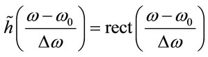 , then according to Equation (5b),
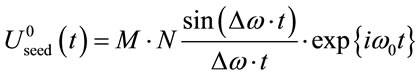 . (38)
If the gain curve is approximated by the Gaussian function (6a)
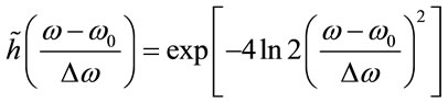
with a spectral width Dw, Eq.(19b), then according to Equation (6b),
 . (39)
5. Conclusion
The sampling and replication operators obtained from the Fourier analysis are elegant and fruitful mathematical tools for the description of the radiation of a modelocked laser. They allowed the effect of the shape of the gain curve of the active medium on the form of the generated UPS to be taken into account.
REFERENCES
- S. Backus, C. G. Durfee, and M. M. Murnane and H. C. Kapteyn, “High Power Ultrafast Lasers,” Review of Scientific Instruments, Vol. 69, No. 3, 1998, pp. 1207-1223. doi:10.1063/1.1148795
- J. Herrman and B. Wilhelmi, “Lasers for Ultrashort Light Pulses,” Akademie, Berlin, 1987.
- S. A. Akhmanov, V. A. Vysloukh and A. S. Chirkin, “Optika Femtosekundnyh Lazernyh Impulsov, (Optics of Femtosecond Laser Pulses, in Russian),” Nauka, Moskva, 1988.
- Wikipedia, the Free Encyclopedia, “Mode-Locking”. http://en.wikipedia.org/wiki/Mode-locking
- H. A. Haus, “Mode-Locking of Lasers,” IEEE Journal of Selected Topics in Quantum Electronics, Vol. 6, No. 6, 2000, pp. 1173-1185. http://wr.lib.tsinghua.edu.cn/sites/default/files/1174986066162.pdf doi:10.1109/2944.902165
- A. M. Weiner, “Ultrafast Optics,” John Wiley & Sons, Inc., Hoboken, 2009. doi:10.1002/9780470473467
- O. Svelto, “Principles of Lasers,” Springer-Verlag, New York, 2009.
- G. Steineyer, D. H. Sutter, L. Gallmann, N. Matuschek, and U. Keller, “Frontiers in Ultrashort Pulse Generation: Pushing the Limits in Linear and Nonlinear Optics,” Science, Vol. 286, No. 5444, 1999, pp. 1507-1512. doi:10.1126/science.286.5444.1507
- F. Träger, “Springer Handbook of Lasers and Optics,” Springer, Berlin, 2007. doi:10.1007/978-0-387-30420-5
- A. Yariv, “Internal Modulation in Multimode Laser Oscillators,” Journal of Applied Physics, Vol. 36, No. 2, 1965, pp. 388-391. doi:10.1063/1.1713999
- U. H. Gerlach, “Linear Mathema tics in Infinite Dimensions,” Columbus, 2009.
- P. Giaccari, J. D. Deschenes, P. Saucier, J. Genest and P. Tremblay, “Active Fourier-Transform Spectroscopy Combining the Direct RF Beating of Two Fiber-Based Mode Locked Lasers with a Novel Referencing Method,” Optics Express, Vol. 16, No. 6, 2008, pp. 4347-4365. doi:10.1364/OE.16.004347
- M. Sheik-Bahae, “Experimental Techniques of Optics,” University of New Mexico, Albuquerque, 2013, http://www.optics.unm.edu/sbahae/Optics%20Lab/index.htm
- W. Wilcock, ESS 522, “Geoscientific Data Analysis, (Outdated Course Catalog Title is “Geophysical Data Collection and Analysis),” 2012. http://www.ocean.washington.edu/courses/ess522/lecturenotes.htm
- G. R. Jiracek, J. F. Ferguson, L. W. Braile and B. Gilpin, “Digital Analysis of Geophysical Signals and Waves”. http://serc.carleton.edu/NAGTWorkshops/geophysics/activities/18990.html
- Wikipedia, the Free Encyclopedia, “Fourier Transform”. http://en.wikipedia.org/wiki/Fourier_transform
- B. Williamson, “The Uncertainty Principle,” 2000. http://users.cecs.anu.edu.au/~williams/uncertainty.pdf
- Wikipedia, the Free Encyclopedia, “Full Width at Half Maximum”. http://en.wikipedia.org/wiki/Full_width_at_half_maximum
- C. Hirlimann, “Laser Basics,” In: C. Rulliere, Ed., Femtosecond Laser Pulses: Principles and Experiments, Springer, Berlin, 2004, pp. 1-23.