Journal of Surface Engineered Materials and Advanced Technology
Vol.1 No.1(2011), Article ID:4272,4 pages DOI:10.4236/jsemat.2011.11001
Finite Element Analysis of the Material’s Area Affected during a Micro Thermal Analysis Applied to Homogeneous Materials
![]()
MAPIEM, EA 4323, Institut des Sciences de l’Ingénieur de Toulon et du Var, Cedex, France
Email: yoann.joliff@univ-tln.fr
Received February 2nd, 2011; revised March 15th, 2011; accepted March 20th, 2011.
Keywords: Micro-Thermal Analysis, Localized Thermal Analysis, Heat Affected Zone, Thermal Conductivity, Finite Element Method
ABSTRACT
Micro-thermal analysis (µ-TA), with a miniaturized thermo-resistive probe, allows topographic and thermal imaging of surfaces to be carried out and permits localized thermal analysis of materials. In order to estimate the effective volume of material thermally affected during this localized measurement, simulations, using finite element method were used. Several parameters and conditions were considered. So, thermal conductivity was found to be the driving physical parameter in thermal exchanges. Indeed, the evolution of the heat affected zone (HAZ) versus thermal conductivity can well be described by a linear interpolation. Therefore it is possible to estimate the HAZ before experimental measurements. This result is an important progress especially for accurate interphase characterization in heterogeneous materials.
1. Introduction
Micro thermal analysis is a characterization technique of thermal and mechanical behaviours of materials at submicroscopic scale [1]. This technique is therefore dedicated to numerous application domains dealing with low scale characterizations such as distinguishing different constituents of a heterogeneous material, identifying the polymorphism or thermal history of polymers, identifying a contaminant or surface film, characterizing interfaces and interphases [2]. Recent technological advances for this technique mainly concern the development of new thermal probes with tip edges that are reduced to the maximum in order to ensure localized measurements [3-5]. The present study aims at estimating the area thermally affected during a localized measurement with the thermal probe (Wollaston wire Pt/Rh). In fact, few works are concerned with this subject which is however crucial for the validity of results, particularly when polymer reinforced composite materials are considered. So, we were interested in developing numerical models that are able to quantify the heat affected zone (HAZ) and to identify parameters that influence its size during localized measurements. The finite element method is used in order to quantify the volume of matter thermally stressed on virtual samples representative of real monophased materials. Therefore, it seems essential to identify physical phenomena (mainly thermal here) that occur during characterization.
The present work describes the technique and discusses the results obtained by this means. Thermal phenomena here above mentioned that have been widely studied in literature these last years will be presented. Then, results obtained from finite element method for the study of the HAZ will be detailed, analyzed and discussed.
2. Micro-Thermal Analysis Process
2.1. Description of the Micro-Thermal Analysis (µ-TA)
The µ-TA experimental device is a Scanning Force Microscope using a miniaturized thermo-resistive probe. The system is composed of four major elements: the thermal probe, a piezo-scanner to control its position in three directions, a thermal control unit and a system for data acquisition. The scanner is linked to a feedback mechanism to maintain a constant force and the probe temperature is controlled by a wheatstone bridge so that an isoforce topographic image and an isothermal apparent thermal conductivity image can be simultaneously recorded. The thermoresistive probe derived from Dinwiddies et al.’s work [6] comprises a Wollaston lever arm at the end of which the Platinum thermoresistive element is fixed. The heating tip is a simple filament of Platinum/10% Rhodium curved in V-shaped (Figure 1) [7].
After positioning the probe on the sample’s surface, a scan is performed at constant force and temperature. Mallarino et al. [8] show an example of apparent thermal conductivity image obtained after scanning a unidirectional glass fibre reinforced composite in transverse direction. Localized thermomechanical measurements intended to determine melting point and glass transition temperature in polymer or composite can then be performed at high temperature rate (10 - 20 K/s) on selected points of the scan. The high rate limits the HAZ dimensions for a given material diffusivity. The probe displacement is then followed versus temperature [8].
In this example, sensor position successively increases showing sample thermal expansion at glassy state, and decreases drastically around 100˚C showing sample softening after glass transition temperature [8].
2.2. Heat Exchange between the Probe and the Sample
The quality of measurements is closely related to the nature of the contact zone between the platinum probe and the surface of the sample. It is therefore important to well-understand the thermal exchanges associated to this localized measurement in order to quantify heat transfers and consequently the HAZ. In a previous work, Shi et al.
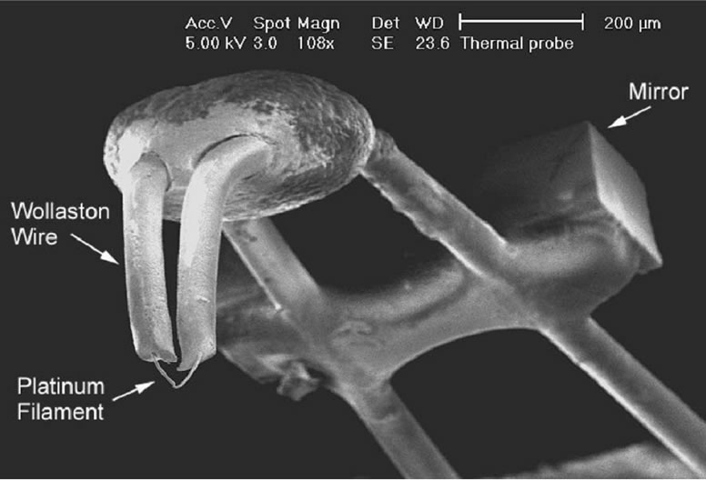
Figure 1. Micrograph of the thermal probe developed by Dinwiddie et al. [6,7]
conducted a detailed study of the thermal mechanisms that take place in the contact area between the thermocouple tip and a hot substrate [9]. Type and shape of the probe and sample, atmospheric environment and distance between the probe and the sample are the parameters to be considered. Existing literature brings back a lot of works [9-11] describing the presence, below 100˚C, of a water meniscus which appears at the periphery of the probe tip and in the cavities created between probe and sample surfaces in the contact zone. In her PhD work [12], Gomes states that the heat exchange through the water meniscus is predominant. The intensity of this exchange is directly linked to the thermal conductivity of the sample.
Consequently, three ways can be considered for describing heat transfers (Figure 2)
o Transfer by conduction (probe/sample and probe/ water/sample);
o Transfer by natural convection (air/sample);
Transfer by radiation (probe/sample).
The involvement of radiation in the heat balance is not significant compared to the natural convection with air [13]. A modelling of the thermal behaviour of the probe of the Scanning Thermal Microscope (SThM) has recently been proposed by Grossel et al. [14]. The thermal exchange along the probe was modelled as a convection gradient of which the heat transfer coefficient value h is maximal at the periphery of the probe/sample contact area (with h = 1200 W/m2/K at the end of the probe in contact with the sample and h = 60 W/m2/K at the other end [15]). A similar study has proposed h values lying between 950 and 1300 W/m2/K [16].
2.3. Contact Area between the Probe and the Sample
The HAZ will closely be related to the size of the contact area between the probe and the sample. Using analytical models, several authors have been able to quantify the dimensions of this contact area. So, Gomes et al. [16]

Figure 2. Different heat transfers mechanisms between the probe and the sample.
estimate a circular contact surface with a 80 nm radius and a concentric circular water meniscus surface with an outside radius of 306 nm. As for Lefèvre et al. [17-19], they have suggested contact radii values ranging from 200 nm to 1 µm depending on temperature and probe geometry.
3. Numerical Approach and Results
Numerical models developed here are based on a 500 nm radius and 1 mm height cylindrical sample (geometrical models have been described by an axisymmetric representation – 2D½). Although the approach presented here is dedicated to study polymer materials, metal and ceramic materials have been chosen for several reasons. First, below 30˚C and 150˚C, their thermal properties can be considered as independent of the temperature. Then, close to 110 - 130˚C, mechanical properties of polymer materials decrease strongly and the thermal probe would push in the sample. So, the contact surface between the probe and the sample increases and must be considered in simulations. These phenomena are not considered here and will be taken into account in a future work where coupled thermomecanical simulations will be used.
Table 1 summarizes the type and properties of the materials that have been studied. Note that theses materials are supposed to be homogenous and isotropic.
The finite element models were realized with Abaqus code and the numerical models are meshed with 400 000 linear axisymetric heat transfer quadrilateral elements. A gradient element size (small: 16 nm × 16 nm / large: 6 × 6 µm) was realized to have a fine discretization under the probe zone.
A transient heat transfer analysis is applied, and heat conduction is assumed to be governed by the Fourier law (Equation (1))
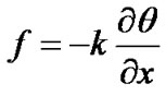 (1)
(1)
with k: matrix of conductivity, k = k(θ)f: heat flux.
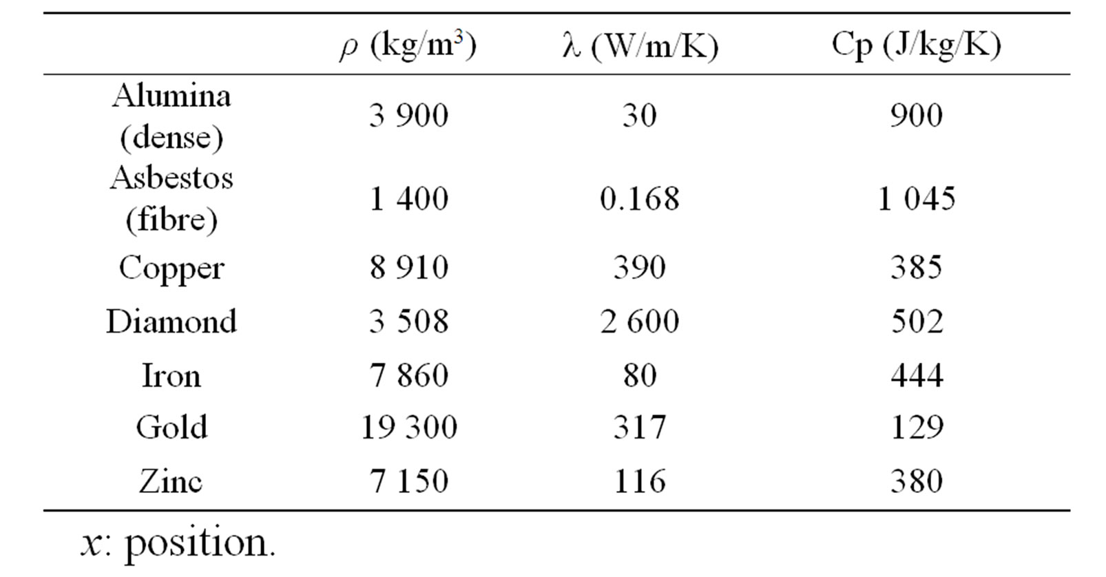
Table 1. Physical properties of materials used for modelling [20].
The thermal probe is replaced by a simplified thermal condition applied to the sample surface: the temperature increase of 15 ˚C/s (thermal loading of the probe) is supposed to be applied on a small surface of the sample equivalent to the probe contact area. The radius of this area is fixed at 80 nm according to the results of Gomes et al. [16] and the presence of the water meniscus is not taken into account in the first step. The initial temperature of the sample is fixed by a prescribed temperature equal to 30˚C. The heat flux q on the top of sample surface due to convection is governed by boundary convection:
 (2)
(2)
with q: heat flux across the surface
h: reference film convection coefficient
θ: temperature at this point on the surface
θ0: reference sink temperature value.
Radiation heat exchange is not taken into account (not significant compared with convection exchange). Figure 3 summarized boundary conditions and thermal loading applied to the model.
The sample is considered as thermally affected if the temperature of the area concerned reaches values higher or equal to 50˚C. The HAZ has been defined as the distance between the centre of the probe and the thermal isovalue of 50˚C in the material. This value of 50˚C was chosen as reference because polymer properties are not affected below glass transition temperature (generally Tg > 60˚C).
3.1. Influence of the Materials Physical Properties on the Zize of the HAZ
Solving the heat transfer equations related to a thermal problem only requires three materials properties: density, thermal conductivity and specific heat. In this part of the study, the aim is to identify the properties that are really influent on the size of the HAZ.
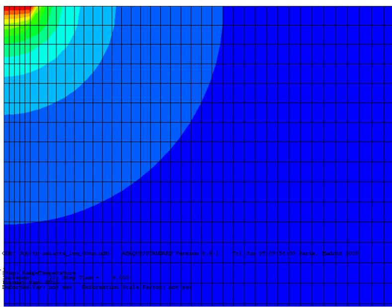
Figure 4 shows the thermal gradient at the end of thermal loading in two samples, a heat insulation (asbestos) and a thermal conductor (copper). The quantity of material thermally impacted is more important in the radial direction than in the longitudinal one. For example, in the case of asbestos, a gap nearing 10% can be calculated between the radial and the longitudinal lengths whereas for copper, the difference is only about 3%. Considering this first result, the shape of the HAZ can therefore be described by a hemispherical shape for thermal conductor materials. While for thermal insulator materials, a hemi-elliptical shape is more appropriate. Later, in this paper, only the radial length on the top surface of the sample is studied.
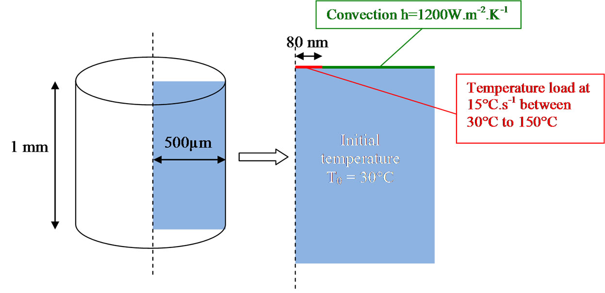
Figure 3. Boundary conditions and thermal load for numerical model.

 (a)
(a) 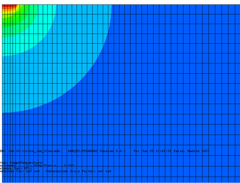 (b)
(b)
Figure 4. Thermal gradient evolution in the sample at the end of thermal loading, i.e. Tprobe = 150˚C for asbestos (a) and copper (b) (zoom in the contact zone with the thermal probe).
Figure 5 presents, at the end of thermal loading (Tprobe = 150˚C), temperature variations along the horizontal upper surface (that is in contact with the probe) of the different model samples. Except for diamond, samples dimensions (1 mm × 1 mm) are enough to define a satisfying representative elementary volume (REV) for modelling µ-TA process. The HAZ is increases with the diffusivity (Figure 6). Moreover, a linear evolution is found between its size and the value of diffusivity.
The evolution of the HAZ versus thermal conductivity can also be well described by a linear interpolation as shown on Figure 7.
The other two parameters, specific heat and density, have been studied as a function of the HAZ (Figure 8 and Figure 9 respectively). It is difficult to use these results to quantify the HAZ since they could not be interpolated by a mathematical function.
3.2. Influence of the Contact Zone
Calculations were carried out by considering different sizes of contact zone for different materials with different
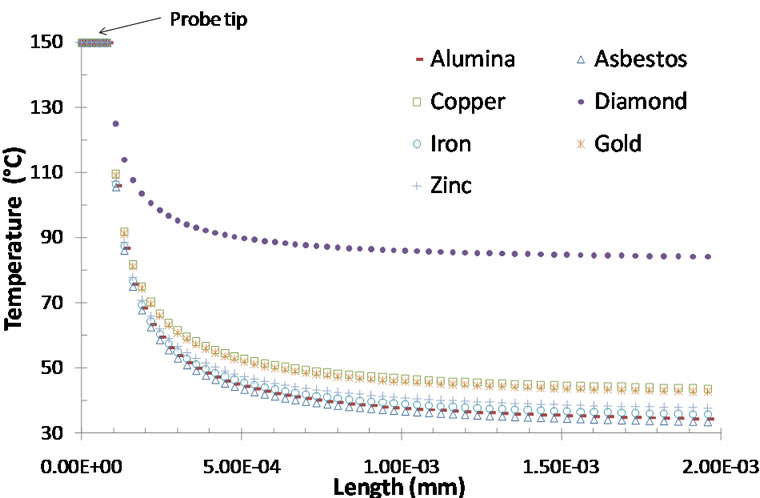
Figure 5. Temperature evolution along the horizontal surface of the sample at the end of thermal loading; i.e. Tprobe = 150˚C (zoom in the contact zone with the thermal probe).
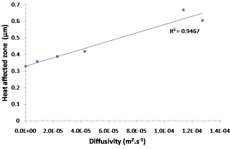
Figure 6. Evolution of heat affected zone versus diffusivity.
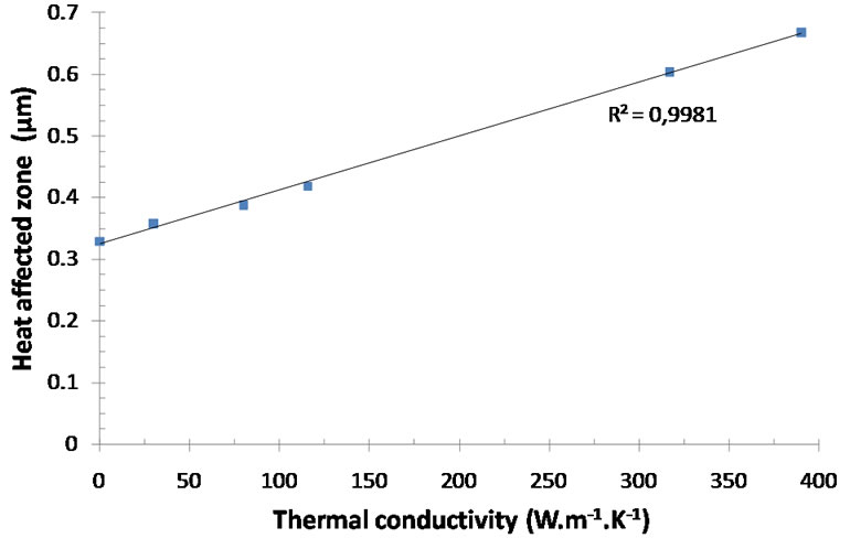
Figure 7. Evolution of heat affected zone versus thermal conductivity.
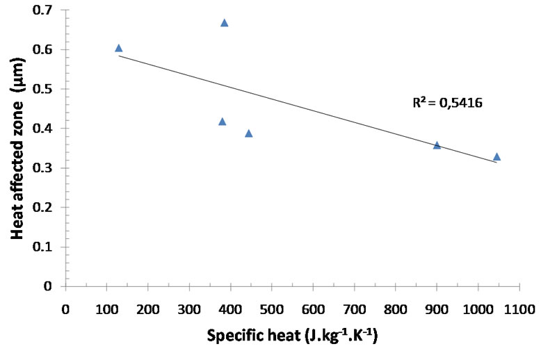
Figure 8. Evolution of heat affected zone versus specific heat.
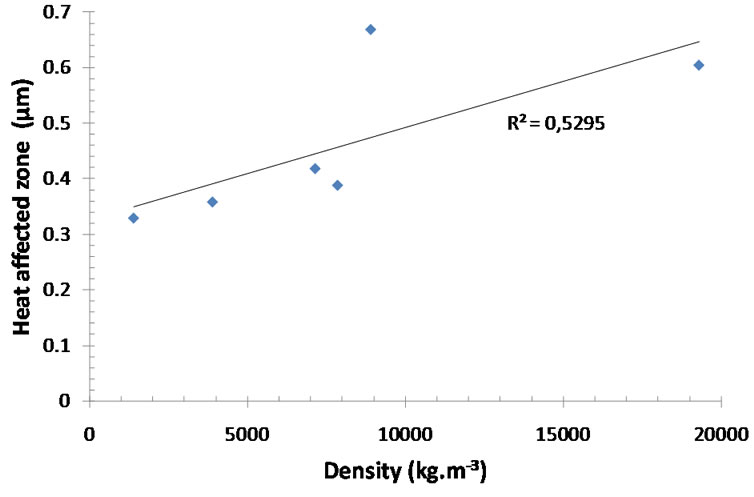
Figure 9. Evolution of heat affected zone versus density.
heat conductivities (copper, zinc, alumina and asbestos). Figure 10 presents the numerical model used for these calculations.
Results are summarized on Figure 11. For thermal insulator materials (asbestos), the increase of the contact
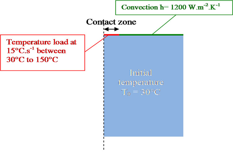
Figure 10. Numerical model used for study of the influence of the contact zone.
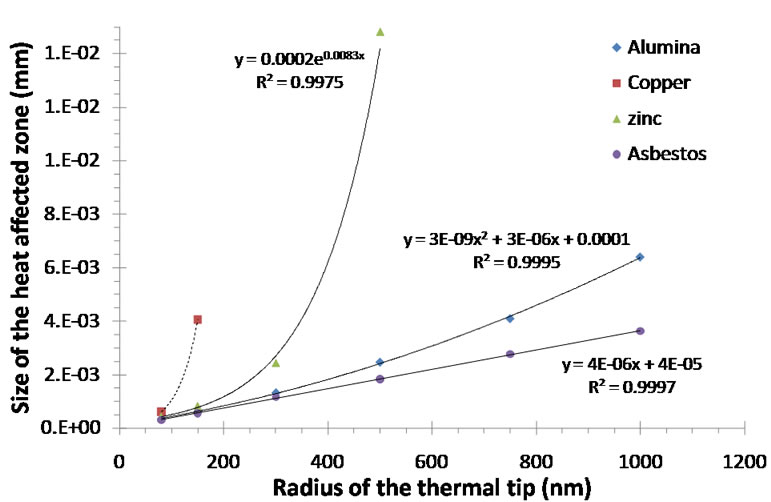
Figure 11. Evolution of heat affected zone versus contact radius between the probe and the sample.
radius leads to a linear increase of the size of the HAZ in the studied temperature range. For heat conductor materials (zinc), the change in HAZ size with temperature is exponential.
3.3. Influence of Water Meniscus
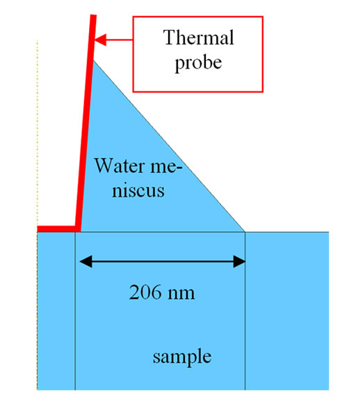
The shape of the probe influences the development of the water meniscus. Three angles are arbitrary fixed for the probe in the study: 15˚, 45˚ and 85˚ (Figure 12). The length of the contact zone between the meniscus and the sample is constant and equal to 206 nm whatever the angle of the probe is [16]. The thermal condition used in previous simulation was applied on a new probe contact area (the sample surface and the water meniscus surface in contact with the thermal probe – Figure 12).
The contact zone between the sample and water meniscus is perfect and no dissipation is allowed. Using the same type of elements as previously, a new meshing was realized. A particular attention was paid to the meshing of the contact zone with thermal probe, and that of water meniscus. Their discretization has been made with small sized elements in order to optimize the results. Boundary conditions and thermal loading applied to numerical models are summarized in Figure 13.
Figure 14 presents the results of the corresponding numerical calculations. From a certain value of thermal conductivity, the role of water meniscus becomes less important. Taking into account the water meniscus in calculations leads to an increase of the HAZ of 27% for alumina and only less than 5% for zinc. On the other hand, when the material has a low thermal conductivity (as for asbestos), the presence of water meniscus leads to an increase of the HAZ from 3 to 5 times depending on the angle of the tip.
4. Discussion
The finite element method enables to determine the influence of intrinsic or external parameters on the size of the zone really thermally affected during a micro thermal analysis (HAZ). The development of simple model representative of matrices with very different thermal properties is enough to define influent parameters such as thermal conductivity. From above results (Figure 7), it should be possible to estimate the size of the HAZ from thermal conductivity measurements after calibrating the μTA on several reference samples of well known thermal conductivities. Concerning specific heat which is difficult to quantify experimentally, no influence has been found on final result.
As expected, the initial contact area of the probe is a critical parameter on final HAZ size as observed on Figure 11. The interest of FEM analysis here is to quantify the influence of contact size on HAZ depending on thermal conductivity. For heat conducting materials, the exponential dependence between contact size and HAZ size requires the smallest possible contact areas. The technological development of micro thermal analysis then needs a miniaturization of this contact zone. As an example, Depasse et al. [21] refer to some 30 nm radius for this zone. This study however deals with an 80 nm radius according to Gomes et al.’s work [10,12,16] that are more successfully completed in regard to the analysis and the understanding of classical micro thermal analysis measurements with standard probes.
Since the probes are handmade, their shapes are heterogeneous, and the results obtained in displacement are therefore dispersed. Moreover, during experiments, these probes are often submitted to irreversible deformations that rapidly modify their initial shapes. The thermal tip usually tends to flatten, leading to the widening either of the angle of the thermal tip or of the angle between the probe and the sample. As mentioned above, this change has a little influence on heat transfer. However, it will be greatly influent during the development of water meniscus that drastically increases the size of the HAZ for heat
 (a)
(a)  (b)
(b)  (c)
(c)
Figure 12. Probes and water meniscus profiles for the different numerical models: probe angle of 85˚ (a), 45˚ (b) and 15˚ (c).

Figure 13. Numerical model used for study of the influence of the water meniscus.
insulator materials (such as asbestos). The thermal conductivity of water is in fact more important than that of the heat insulator material, what interferes with localized measurements. It is therefore fundamental to take this phenomenon into account for this materials family.
5. Conclusions
Making localized characterization is usually difficult to obtain. The physical parameters and the behaviours of materials are in fact modified compared to the macroscopic scale. So, it is an important challenge to be able to quantify at this small scale the thermal and mechanical stresses occurring on materials. Using numerical simulation and considering the heat insulator or conductor materials, this work led to the quantification of the heat affected zone during a localized micro thermal analysis. From the study of several parameters and conditions, the thermal conductivity has been found to be the driving physical parameter in thermal exchanges. It has therefore been possible to rapidly estimate the heat affected zone. Models showed that the water meniscus that appears at the interface between the probe and the sample has only little influence on the size of the heat affected zone for heat conductor materials. On the contrary, for heat insulator materials, this meniscus can lead to an increase of the size of the heat affected zone from 3 to 5 times. The contact angle has a limited influence on conductor materials and a higher influence on insulators. Finally, owing

Figure 14. Evolution of heat affected zone for different shapes of probe and water meniscus.
to their varying shapes coming from diversified technological developments, the probes will probably modify the water meniscus and the size of the heat affected zone.
This work is just a first study on the topic of heat affected zone. In a near future, it will be necessary to complete it by defining new models that would describe multiphased materials and to quantify the corresponding heat affected zones surrounding different phases.
REFERENCES
- E. Gmelin, R. Fischer and R. Stitzinger, “Sub-Micrometer Thermal Physics—An overview on STHM Techniques,” Thermochimica Acta, Vol. 310, No. 1-2, 1998, pp. 1-17. doi:10.1016/S0040-6031(97)00379-1
- H. M. Pollock and A. Hammiche, “Micro-Thermal Analysis: Techniques and Applications,” Journal of Physics D: Applied Physics, Vol. 34, 2001, pp. R23-R53. doi:10.1088/0022-3727/34/9/201
- A. Altes, R. Tilgner and W. Walter, “Numerical Evaluation of Miniaturized Resistive Probe for Quantitative Thermal Near-Field Microscopy of Thermal Conductivity,” Microelectronics Reliability, Vol. 46, No. 9-11, 2006, pp. 1525-1529. doi:10.1016/j.microrel.2006.07.030
- I. W. Rangelow, T. Gotszalk, N. Abedinov, P. Grabieca and K. Edingerb, “Thermal Nano-Probe,” Microelectronic Engineering, Vol. 57-58, 2001, pp. 737-748. doi:10.1016/S0167-9317(01)00466-X
- D.-W. Lee and I.-K. Oh, “Micro/Nano-Heater Integrated Cantilevers for Micro/Nano-Lithography Applications,” Microelectronic Engineering, Vol. 84, No. 5-8, 2007, pp. 1041-1044. doi:10.1016/j.mee.2007.01.104
- R. Dinwiddie, R. Pylkki and P. West, “Thermal Conductivity Contrast Imaging with a Scanning Thermal Microscope,” Thermal Conductivity, Vol. 22, 1994, pp. 668-677.
- P. G. Royall, V. L. Kett and C. S. Andrews and D. Q. M. Craig, “Identification of Crystalline and Amorphous Regions in Low Molecular Weight Materials Using Microthermal Analysis,” The Journal of Physical Chemistry B, Vol. 105, 2001, pp. 7021-7026. doi:10.1021/jp010441k
- S. Mallarino, J. F. Chailan and J. L. Vernet, “Interphase Investigation in Glass Fibre Composites by Micro-Thermal Analysis,” Composites Part A: Applied Science and Manufacturing, Vol. 36, No. 9, 2005, pp. 1300- 1306. doi:10.1016/j.compositesa.2005.01.017
- L. Shi and A. Majumdar, “Thermal Transport Mechanisms at Nanoscale Point Contacts,” Journal of Heat Transfer, Vol. 124, 2002, pp. 329-337. doi:10.1115/1.1447939
- S. Gomés, N. Trannoy and P. Grossel, “D.C. Thermal Microscopy: Study of the Thermal Exchange between a Probe and a Sample,” Measurement Science and Technology, Vol. 10, No. 9, 1999, pp. 805-811.
- S. Lefèvre, “Modélisation et Élaboration des Métrologies de Microscopie Thermique à Sonde Locale Résistive,” Ph.D. Dissertation, Poitiers University, Poitiers, 2004.
- S. Gomes, “Contribution Théorique et Expérimentale à la Microscopie Thermique à Sonde Locale: Calibration d’Une Pointe Thermorésistive, Analyse des Divers Couplages Thermiques,” Ph.D. Dissertation, Reims University, Reims, 1999.
- S. Lefèvre, S. Volz and P. O. Chapuis, “Nanoscale Heat Transfer at Contact between a Hot Tip and a Substrate,” International Journal of Heat and Mass Transfer, Vol. 49, No. 1-2, 2006, pp. 251-258.
- P. Grossel, O. Raphaël, F. Depasse, T. Duvaut and N. Trannoy, “Multifrequential AC Modeling of the SThM Probe Behaviour,” International Journal of Thermal Sciences, Vol. 46, No. 10, 2007, pp. 980-988. doi:10.1016/j.ijthermalsci.2006.12.004
- V. T. Morgan, “The Overall Convective Heat Transfer from Smooth Circular Cylinders,” Advances in Heat Transfer, Vol. 11, 1975, pp. 199-264. doi:10.1016/S0065-2717(08)70075-3
- S. Gomes, N. Trannoy, P. Grossel, F. Depasse, C. Bainier and D. Charraut, “D.C. Scanning Thermal Microscopy: Characterization and Interpretation of the Measurement,” International Journal of Thermal Sciences, Vol. 40, 2001, pp. 949-958. doi:10.1016/S1290-0729(01)01281-9
- S. Lefèvre, S. Volz, J.-B. Saulnier, C. Fuentes and N. Trannoy, “Thermal Conductivity Calibration for Hot Wire Based DC Scanning Thermal Microscope,” Review of Scientific Instruments, Vol. 74, No. 4, 2003, pp. 2418-2423.
- S. Lefèvre, J.-B. Saulnier, C. Fuentes and S. Volz, “Probe Calibration of the Scanning Thermal Microscope in the AC Mode,” Vol. 35, No. 3-6, 2004, pp. 283-288.
- S. Lefèvre and S. Volz, “3ω-Scanning Thermal Microscope,” Review of Scientific Instruments, Vol. 76, No. 3, 2005, pp. 033701-033701-6.
- F. Cardarelli, “Materials Handbook—A Concise Desktop Reference,” 2nd Edition, Springer-Verlag London, 2008.
- F. Depasse, P. Grossel and N. Trannoy, “Probe Temperature and Output Voltage Calculation for the SThM in A.C. Mode,” Superlattices and Microstructures, Vol. 35, No. 3-6, 2004, pp. 269-282. doi:10.1016/j.spmi.2004.01.008