Geomaterials
Vol.3 No.2(2013), Article ID:30847,7 pages DOI:10.4236/gm.2013.32006
Roughness Research of Center Profile Curve on Rock Fracture Surface Based on Statistical Method
1School of Mathematics, Nanjing Normal University, Taizhou College, Taizhou, China
2State Key Laboratory of Coal Resources and Safe Mining, China University of Mining and Technology, Beijing, China
3Faculty of Science, Jiangsu University, Zhenjiang, China
4Faculty of Civil Engineering and Mechanics, Jiangsu University, Zhenjiang, China
Email: xzpan1975@yahoo.com.cn, *zgfeng@ujs.edu.cn, daigx@163.com, honggliu@ujs.edu.cn
Copyright © 2013 Xuezai Pan et al. This is an open access article distributed under the Creative Commons Attribution License, which permits unrestricted use, distribution, and reproduction in any medium, provided the original work is properly cited.
Received January 4, 2013; revised February 2, 2013; accepted February 16, 2013
Keywords: Rock Mechanics; Rock Fracture Surfaces; Normal Vector; Statistics; Normal Distribution
ABSTRACT
In order to research roughness of rock fracture surfaces whether to depend on scale effect, Brazil discs were fractured under tensile and compression stresses in Brazil split test with MTS (Mechanics Test Systems) and a laser profilometer was used to scan rock fracture surfaces and coordinates datum of central profile were acquired. A figure of the central profile was plotted through the coordinates datum. A certain line segment length is regarded as a step length, which is called scale and the scale length is taken to connect pairs of closer peak points on the profile curve. The directional distribution of every scale’s normal vector is analyzed by statistics and normal hypothesis test. Finally, some statistics of sample degrees datum are compared with other ones and reach a conclusion that roughness of center profile curve depends on scale effect. The distribution of degrees more and more approximates normal distribution along with increase of scale.
1. Introduction
Deformity and fracture of rock are involved in process of moving in earth crust, for example, earthquake, slide downhill, mud-stone flow and so on. In addition, rock fracture usually happens in rock project, for instance, explosion of rock, the project of tunnel, mining engineering etc. Studying rock fracture surfaces through morphology has been recognized by professionals since twenty-one century, because morphology of rock fracture surfaces implicates abundant information of rock fracture mechanics. Experts have discovered that rock fracture surface has characterization of roughness, irregularity and complexity. They attempt to depict the relation between complex morphology of rock fracture surfaces and roughness by all kinds of ways. For example, In order to assess the current state of rock masses and to predict the stability of jointed rock structures, the roughness of rock fracture surfaces has been studied to a higher level. Based on systematic experiments, Barton and Choubey in 1977 proposed a conceptual model to quantify the roughness of rock fracture surface [1]. They classified the roughness into ten categories and the Joint Roughness Coefficients (JRC) ranged from 0 to 20 [2-4]. Some investigators use fractal geometry and multifractal which have been developed since 1970’s to describe rock fracture mechanism and have tried to establish the relationship between the fractal dimension and various mechanical parameters of rock fracture surfaces [5-8]. Some experts have indicated that the structural anisotropy of fracture surfaces in rocks greatly influences the mechanical behavior of rock joints under loading [9-11]. The following statement will study roughness of center profile curve on rock fracture surfaces from statistical view. Finally, three prospects will be put forward in the end of the paper.
2. Experimental Method and Analysis
2.1. Experimental Method
Firstly, a sort of special granites which were taken from Gansu province north mountain in China were used to experimental material, because the compactness of the rock material is relatively homogeneous. The granite material was made of the cylinder-shaped sample with rock drilling machine, and then the cylinder-shaped sample was cut into three Brazil discs samples with cutting off machine and buffing machine. The diameter and the height of the discs are equal to 112 mm and 28 mm respectively. Secondly, the rock discs were fractured under tensile and compression stresses in Brazil split test with MTS (Mechanics Test Systems). Loading speed was perminute 0.01 mm. When loading strength approximatively reaches 48 kN, the discs were fractured along vertical direction (refer with: Figure 1). Finally, according to rock mechanics principle, in indirect tensile stresses process of rock, the rock stress of the edge of disc is relatively centralized, so the edge of the disc was easily broken and a little stone chips fell. Whereas inner stress of the rock disc is relatively balanced [12-13], the inner of fracturerock has no stone chips fallen. So, 11 mm was removed from two ends of the rectangular fracture surfaces respectively. The length of center part of fracture surface is equal to 90 mm (refer with: Figure 2). The length of 90 mm is supposed to x axis direction. The center part of fracture surface was scanned by high-accuracy rock laser
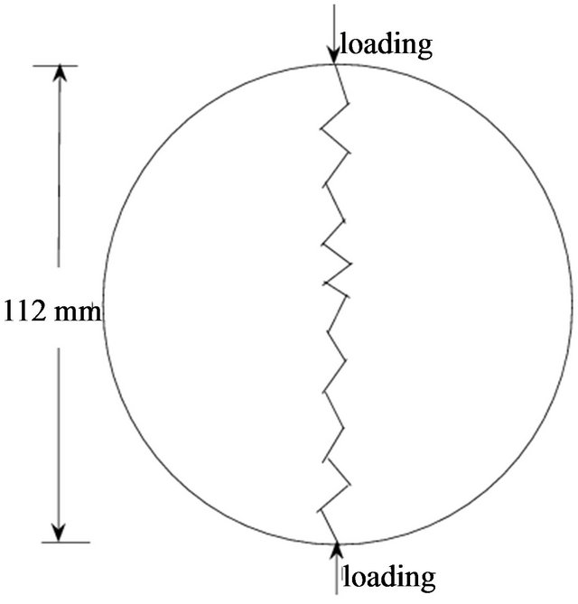
Figure 1. Indirect tensile diagrammatic sketch.
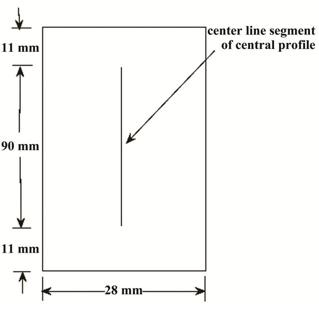
Figure 2. Center profile acquired datum.
profilometer along x axis according to the way that interval of x axis is equal to 0.1 mm to acquired three dimension coordinates (x, y, z) of lattice. Total 901 rope line segments were scanned through the above method, because the length of center part of fracture surface is 90 mm. Length of every line segment scanned is 28 mm, since the width of center part of rock fracture surface is equal to 28 mm (refer with: Figure 2).
2.2. Center Profile Curve Analysis on Rock Fracture Surface
The coordinates datum of the center segment of central profile curve on rock rectangle fracture surface (refer with: Figure 2) was extracted by computer procedure, and then the approximative two dimension curve figure of the profile was acquired by linear interpolating method (refer with: Figure 3). A unit length of step length is supposed to 0.1 mm. A step length was taken to connect pairs of points on the center profile [14-16]. Normal vectors’ directional distribution of corresponding step length was considered and every angle of each normal vector departing from straight up vector is measured (refer with: Figure 4).The motivation for this approach is straightforward: for a perfectly straight profile the normal vectors will all be parallel and hence display zero dispersion, whereas the dispersion will increase as the profile departs from straight (i.e. becomes rougher). Suppose angle of straight up vector is zero degree. The degree of the angle in the direction skewing to left is negative, whereas that skewing to right is positive. Thus, these degree datum of angles can be obtained with computer procedure.
3. Statistical Method
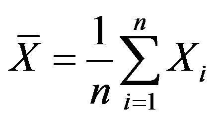
From statistical knowledge [17-20], mean and median of sample (refer with: Equation (1)) reflect concentrated
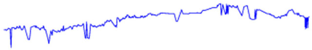
Figure 3. Linear interpolating figure of center profile.
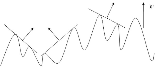
Figure 4. Orientation of normal vector to a step length connecting two points on a profile curve.
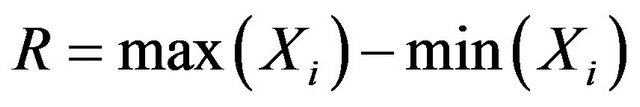
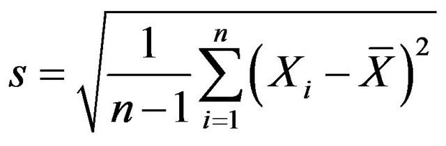
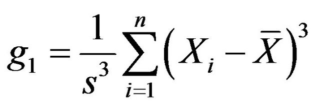
tendency of sample datum. Range (refer with: Equation (2)), variance and sample standard deviation (refer with: Equation (3)) indicate the extent that sample datum depart from sample mean. Skewness (refer with: Equation (4)) and kurtosis (refer with: Equation (5)) are such statistic describing the shape of sample datum. Skewness reflects dispersive symmetrical characterization of sample datum. Finally, kurtosis indicates the situation that sample datum deviate normal distribution.
 (1)
(1)
 (2)
(2)
 (3)
(3)
 (4)
(4)
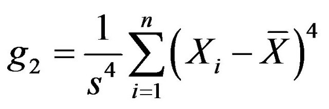 (5)
(5)
where  denotes samples.
When g1 > 0, the form is called right deviation, which illustrates the right datum of mean are more dispersive than those of the left datum; As g1 < 0, the result is named left deviation, which illustrates the situation is opposite to that of right deviation. As g1 approach zero, which is called impartiality, So, the distribution is regarded as symmetry. On the other hand, kurtosis of normal distribution is equal to 3. As g2 > 3, there are a lot of datum departing from mean, whose shape of distributive curve is flatter than that of normal distribution accordingly; On the contrary, when g2 < 3, the case is inverse to that of g2 > 3. So, statistical method can be used to characterize roughness of profile curve subjected to fracture surfaces. The following discussion is concrete operation.
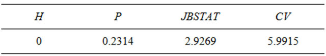
Suppose the step length is equal to 0.4 mm, 0.3 mm, 0.2 mm and 0.1 mm respectively, then the datum of angle variation are acquired by computer procedure corresponding to various step length. Furthermore, under the same scale, sample mean, median, range, variance, standard deviation, coefficient of skewness and kurtosis are computed respectively and frequency histogram [21-25] is drawn with computer program, which describes the distribution of orientation of normal vectors from the center profile curve. Frequency histogram under a step length is compared with that of other ones, which can show distributional differences each other. On the other hand, hypothesis test method is used to test whether the distribution of normal vectors obeys normal distribution or not and distribution function plots were drawn with computer program. For the degree datum input into computer, Jarque-Bera test is used to test these degree datum whether to obey normal distribution. Significance level ![]() is supposed to 0.05. P is a probability value accepting original hypothesis. JBSTAT is test statistics value. CV is a threshold which can judge whether to refuse original hypothesis and H is test result. If H = 0, the distribution of the degree datum can be considered normal distribution; If H = 1, the distribution of the degree datum doesn’t obey normal distribution. If
is supposed to 0.05. P is a probability value accepting original hypothesis. JBSTAT is test statistics value. CV is a threshold which can judge whether to refuse original hypothesis and H is test result. If H = 0, the distribution of the degree datum can be considered normal distribution; If H = 1, the distribution of the degree datum doesn’t obey normal distribution. If , original hypothesis that the datum belong to normal distribution can be denied; If JBSTAT > CV, normal distributional original hypothesis can be negated. Every statistic in following tables is a mean value of corresponding statistic of three center profile curves datum under the same step length (i.e. the same scale), because there are three Brazil discs samples. The differences among the same statistic are compared within four tables under different scales.
1) If the step length is equal to 0.4 mm, the following Tables 1 and 2 indicate a statistical result.
In Table 1, unit of mean, median, range and standard deviation is degree, whereas other statistics have no unit, because they are only coefficients (below affinity).
Variables in Table 2 have no unit (below affinity). From coefficient of skewness −0.0013 ( ), dispersive extent of datum with left side and right one deviating mean is almost comparative. Distribution of angles’ degrees approximatively summits to normal distribution from kurtosis coefficient 3.1511 (
 ) and its frequency histogram is referred with Figure 5. From hypothesis test view, where H = 0,
  and JBSTAT < CV, the normal distributional original hypothesis can be accepted. From normal probability plot shown in Figure 6, the absolute major points gather on the red straight line, which illustrates the normal distributional suppose can be accepted.
In Figure 5, i denotes positive integer and 1 ≤ i ≤ 12, because frequency histogram consists of twelve columns.

Figure 5. The histogram with the step length 0.4 mm (θ: degree; fi(θ): frequency).
Table 1. Statistics of sample datum with the step length 0.4 mm.

Figure 6. Normal probability plot with the step length 0.4 mm (θ: degree; p(θ): probability).
Table 2. Hypothesis test value with the step length 0.4 mm.
2) If the step length is equal to 0.3 mm, the statistical datum result is shown in the Tables 3 and 4.
The extent of departing from sample mean increases; The skewness coefficient increases and is more than 0, which illustrates the right datum of mean is more dispersive than that of the left, but the dispersive extent is faint; Kurtosis coefficient is equal to 2.8296 ( ), which illustrates distribution of angle datum approximate normal distribution. The frequency histogram reflects that the distribution of angle datum close to normal distribution (shown in Figure 7). From normal hypothesis test view, H = 0, P = 0.6492 and JBSTAT < CV indicate normal distributional hypothesis can be accepted with 64.92% probability. From normal probability plot shown in Figure 8, the absolute major points gather on the red straight line, which illustrates the normal distributional suppose can be accepted.
3) If the step length is equal to 0.2 mm, the statistical result is shown in the next Tables 5 and 6.
The sample mean and median increase; Variance and standard deviation increase furthermore; Range hardly change; Coefficient of skewness reduces, however the decrement is very little; coefficient of kurtosis decreases furthermore and reaches 1.9127, which illustrates the distribution of angle datum continues to deviate from normal
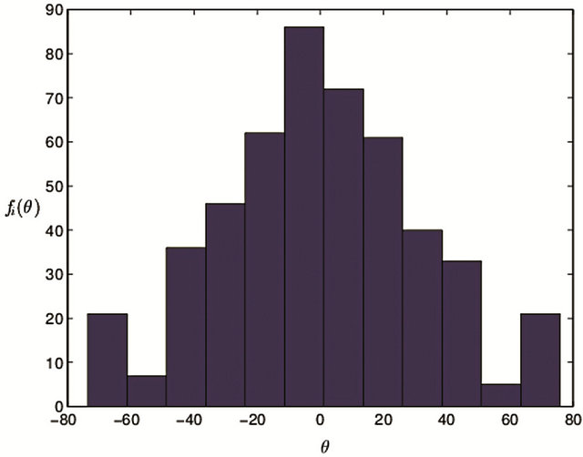
Figure 7. The histogram with the step length 0.3 mm (θ: degree; fi(θ): frequency).
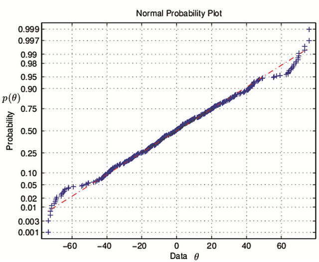
Figure 8. Normal probability plot with the step length 0.3 mm (θ: degree; p(θ): probability).
distribution. Frequency histogram is shown in Figure 9. From normal hypothesis test view, H = 1, the value of P and JBSTAT > CV indicate normal distributional hypothesis can be negated. Normal probability plot is referred with Figure 10.
4) If the step length is equal to 0.1 mm, the following Tables 7 and 8 indicate according statistical result.
The value of sample mean and median has a weak variation; Range still change rarely; Variance and standard deviation increase greatly; Coefficient of skewness continues to decrease, but it still fluctuates near 0, which still describes that two sides’ datum of mean have the same dispersion characterization; Coefficient of kurtosis de
Table 3. Statistics of sample datum with the step length 0.3 mm.

Table 4. Hypothesis test value with the step length 0.3 mm.

Table 5. Statistics of sample datum with the step length 0.2 mm.

Table 6. Hypothesis test value with the step length 0.2 mm.

Table 7. Statistics of sample datum with the step length 0.1 mm.

Table 8. Hypothesis test value with the step length 0.1 mm.
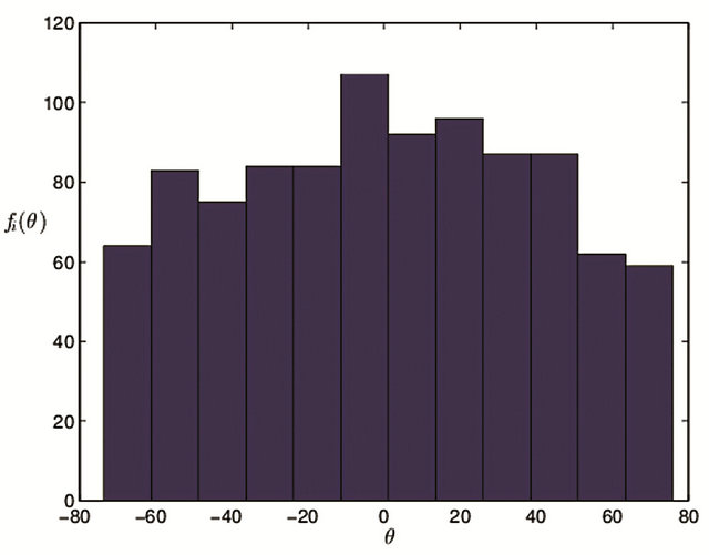
Figure 9. The histogram with the step length 0.2 mm (θ: degree; fi(θ): frequency).
scends further and attains 1.6600, which indicates that the distribution of normal vector deviates from normal distribution; Frequency histogram is shown in Figure 11. From normal hypothesis test view, H = 1, the value of P = 0 and JBSTAT ![]() CV indicate normal distributional
CV indicate normal distributional
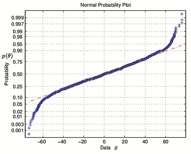
Figure 10. Normal probability plot with the step length 0.2 mm. (θ: degree; p(θ): probability).
hypothesis can be negated completely. Normal probability plot is referred with Figure 12.The absolute major points deviates from the red straight line.
In conclusion, the directional distribution of normal
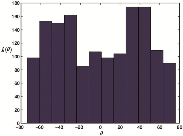
Figure 11. The histogram with the step length 0.1 mm (θ: degree; fi(θ): frequency).
vectors is associated with the step length, which depends on scale effect. The smaller the kurtosis is, the smaller the scale is, which illustrates the distribution of angle datum deviates from normal distribution continuously. The case that range of sample datum is close to 149 is disco vered, which indicates that variable range of angle degrees is definite. And the dispersive extent between the left datum of sample mean and those of right is comparative, because skewness coefficient is almost equal to 0. In summary, the roughness of center profile curve could be supposed to standard state, when the distribution of angle datum belongs to standard normal distribution. Furthermore, the rougher center profile curve is, the smaller the step length is.
4. Conclusion and Prospect
In generally, mean, median, range and skewness coefficient almost have no scale effect, however, variance and standard deviation will increase with decreasing of scale. Kurtosis coefficient will descent along with diminishing of scale. Accordingly, from normal hypothesis test view, H, P, JBSTAT have scale effect too. As a whole, H leaps from 0 to 1 along with decreasing of scale. P will decrease while scale drops. JBSTAT will raise as scale falls. That is to say, the rougher center profile curve is, the smaller the step length is. The ultimate purpose of researching morphology of rock fracture surfaces is that the information in process of rock fracture is acquired through methods of mathematical analysis. Successively, components of rock structure and limitation are discovered and further mechanics of rock fracture is posted. However, structure of rock and properties of mechanics exhibit nonlinear characterization. Rock fracture surface possesses fairly irregular and stochastic properties, hence the topic is developed so slowly that the results acquired through researching haven’t been applied in forecasting and instructing practise of project. Therefore, the follow-
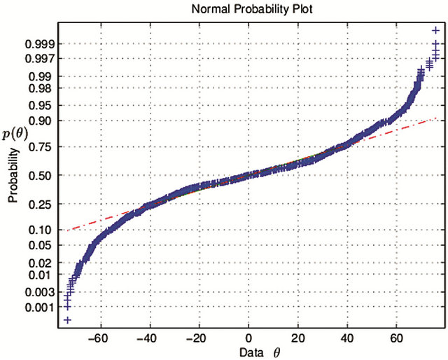
Figure 12. Normal probability plot with the step length 0.1 mm (θ: degree; p(θ): probability).
ing three aspects of research will be evolved. Firstly, advantages of approaches applied by experts now continue to be developed and perfected, and insufficiencies will be overcome extensively, which attempt to build the relationship between rock mechanics and topograph of rock fracture surfaces. Secondly, new approaches of studying rock fracture surfaces through morphology will be sought, which try to discover the mechanics of rock fracture. Finally, existing experimental results will be transformed into theoretical basis of guiding project practice possibly.
5. Acknowledgements
1) Supported by the National Natural Science Foundation of China 51079064.
2) Supported by State Key Laboratory of Coal Resources and Safe Mining, China University of Mining and Technology SKLCRSM10KFA02.
3) Supported by Nanjing Normal University Taizhou College Q201234.
REFERENCES
- N. Barton and V. Choubey, “The Shear Strength of Rock Jounts in Theory and Practice,” Rock Mechanics, Vol. 1977, Vol. 10, No. 2, pp. 1-45. doi:10.1007/BF01261801
- N. Barton, “Review of a New Shear Strength Criterion for Rock Joints,” Engineering Geology, Vol. 7, No. 4, 1973, pp. 287-332. doi:10.1016/0013-7952(73)90013-6
- R. Tse and D. M. Cruden, “Estimating Joint Roughness Coefficients,” International Journal of Rock Mechanics and Mining Sciences & Geomechanics Abstracts, Vol. 16, No. 5, 1979, pp. 303-307. doi:10.1016/0148-9062(79)90241-9
- N. H. Maerz, J. A. Franklin and C. P. Bennett, “Joint Roughness Measurement Using Shadow Profilometry,” International Journal of Rock Mechanics and Mining Sciences & Geomechanics Abstracts, Vol. 27, No. 5, 1990, pp. 329-343. doi:10.1016/0148-9062(90)92708-M
- K. Falconer and W. G. Yang, “Fractal Geometry Mathematical Foundations and Applications,” 2nd Edition, Posts & Telecom Press, Beijing, 2007.
- Y. H. Zhang, H. W. Zhou and H. P. Xie, “Improved Cubic Covering Method for Fractal Dimensions of a Fracture Surface of Rock,” Chinese Journal of Rock Mechanics and Engineering, Vol. 24, No. 17, 2005, pp. 3192- 3196.
- H. P. Xie, H. Q. Sun, Y. Ju, et al., “Study on Generation of Rock Surfaces by Using Fractal Interpolation,” International Journal of Solid and Structure, Vol. 38, No. 32-33, 2001, pp. 5765-5787. doi:10.1016/S0020-7683(00)00390-5
- H. P. Xie, J.-A. Wang and M. A. Kwa Niewski, “Multifractal Characterization of Rock Fracture Surfaces,” International Journal of Rock Mechanics Mining Sciences, Vol. 36, No. 1, 1999, pp. 19-27. doi:10.1016/S0148-9062(98)00172-7
- S. C. Bandis, A. C. Lumsden and N. R. Barton, “Fundamentals of Rock Joint Deformation,” International Journal of Rock Mechanics and Mining Sciences & Geomechanics Abstracts, Vol. 20, No. 6, 1983, pp. 249-268. doi:10.1016/0148-9062(83)90595-8
- P. H. S. W. Kulatilake, G. Shou, T. H. Huang and R. M. Morgan, “New Peak Shear Strength Criteria for Anisotropic Rock Joints,” International Journal of Rock Mechanics and Mining Sciences & Geomechanics Abstracts, Vol. 32, No. 7, 1995, pp. 673-697. doi:10.1016/0148-9062(95)00022-9
- H. W. Zhou and H. Xie, “Anisotropic Characterization of Rock Fracture Surfaces Subjected to Profile Analysis,” Physics Letters A, Vol. 325, No. 5-6, 2004, pp. 355-362. doi:10.1016/j.physleta.2004.04.006
- W. Gao, “Mechanics of Rock,” Peking University Press, Beijing, 2010.
- Z. L. Fu, F. K. Xiao, Y. X. Liu and S. J. Chen, “Experiment Course on Rock Mechanics,” Chemistry Engineering Press, Beijing, 2010.
- V. Rasouli and J. P. Harrison, “Assessment of Rock Fracture Surface Roughness Using Riemannian Statistics of Linear Profiles,” International Journal of Rock Mechanics Mining Sciences, Vol. 47, No. 6, 2010, pp. 940-948. doi:10.1016/j.ijrmms.2010.05.013
- V. Rasouli and J. P. Harrison, “Scale Effect, Anisotropy and Directionality of Discontinuity Surface Roughness,” Proceedings of the EUROCK Symposium, Aachen, 27-31 March 2000, pp. 751-756.
- T. H. Wu and E. M. Ali, “Statistical Representation of Joint Roughness,” International Journal of Rock Mechanics and Mining Science & Geomechanics Abstracts, Vol. 15, No. 5, 1978, pp. 259-262. doi:10.1016/0148-9062(78)90958-0
- Z. S. Wei, “Probability and Statistics Tutorial,” Higher Education Press, Beijing, 1983.
- X. R. Chen, “Higher Statistics,” China University of Science and Technology, Hefei, 1999
- G. X. Liu, Z. F. He and J. L. Yang, “Probability and Statistics,” Gansu Education, Lanzhou, 2002.
- X. S. Liu, “Probability and Statistics,” Sichuan University Press, Chengdu, 2009.
- L. B. Wu and B. N. Li, “Mathematical Experiment and Modeling,” Defense Industry Press, Changsha, 2007.
- J. Zhao and Q. Dan, “Mathematical Modeling and Mathematical Experiment,” Higher Education Press, Beijing, 2000.
- H. G. Zhang, “Practical Tutorial of MATLAB/SIMULINK,” Posts & Telecom Press, Beijing, 2009.
- D. X. Zhang and L. S. Zhao, “Teaching of Language Procedure Design of MATLAB,” China Railway Press, Beijing, 2010.
- P. Wu, “Technology and Application of Effective Procedure of MATLAB: Analysis of 25 Cases,” Beihang University Press, Beijing, 2010.
NOTES
*Corresponding author: Tel: +86 511 88791138.