Received 21 February 2016; accepted 24 April 2016; published 27 April 2016

ABSTRACT

This paper investigates the effect of inflow, outflow and shock waves in a single lane highway traffic flow problem. A constant source term has been introduced to demonstrate the inflow and outflow. The classical Lighthill Whitham and Richards (LWR) model combined with the Greenshields model is used to obtain analytical and numerical solutions. The model is treated as an IBVP and numerical solutions are presented using Lax Friedrichs scheme. Godunov method is also used to present shock wave analysis. The numerical procedures adopted in this investigation yield results which are very much consistent with real life scenario in terms of traffic density and velocity.

Keywords:

Macroscopic Model, Source Term, Shock Wave, Lax Friedrichs Scheme, Godunov Method

1. Introduction

The problem of traffic congestion is becoming endemic due to increased levels of population. Traffic conditions in many major metropolitan areas are becoming increasingly congested, affecting the operational efficiency of whole networks as well as the travel cost of each trip. Therefore, traffic flow models are becoming more important in traffic engineering and the transportation policy making process. In an effort to minimize congestion, an accurate method for modeling the flow of traffic is imperative. Mainly two approaches are widely used in describing traffic flow phenomena mathematically. The first one is the microscopic model which describes flow by tracking individual vehicles using car-following logic. On the other hand, macroscopic models are concerned with describing the flow-density relationship for a traffic stream (a group of vehicles). Macroscopic models are more suitable for modeling traffic flow since less supporting data and computation are needed. In this paper, we have studied macroscopic traffic flow models.

Computer simulation of traffic is a widely used method in research of traffic modeling, planning and development of traffic networks and systems. Many research groups are involved in dealing with the problem with different kinds of traffic models for several decades [1] - [3] . In most cases, the source terms that have been appeared in traffic flow equations [4] [5] represent inflow and outflow in a single-lane highway. In this paper, some necessary modifications have been made in existing macroscopic models to represent the effect of constant rate inflow and outflow. This analysis also focuses on the existence and propagations of stationary shock waves. The approximation of scalar conservation laws is carried out by using conservative methods, such as the Lax- Friedrichs scheme and classical Godunov scheme with the use of suitable initial and boundary conditions.

2. Mathematical Modeling and Procedures

If a vehicle in a single lane highway can be assumed to be a molecule, then the traffic can be defined to be an incompressible fluid which cannot be compressed after a certain density. In 1955 and 1956, Lighthill, Whitham and Richards proposed a macroscopic traffic flow model which is known as the LWR model [6] . According to this model, the traffic flow is represented using a first order partial differential equation. Based on a hyperbolic system of conversation laws, this equation is defined as following:

(1)

where is the density of cars and denote the traffic flow rate (flux) all of which are functions of space, and time,. Flux can be written as the product of the density and of the mean velocity of the cars, i.e.. Inserting this relationship in (1), we obtain

(2)

A linear relationship between velocity and density proposed by Greenshields [7] is given by the following equation:

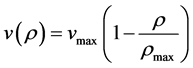(3)

where is the maximum velocity and is the maximum density of the road. This specific relationship between traffic velocity, flux and density is presented in Figure 1. According to [8] , inserting the linear velocity- density closure relationship (3) into (2), we obtain the specific first order non-linear partial differential equation of the form:

(4)

2.1. Role of Source Term in Traffic Flow Models

A source term in the Equation (4) for the vehicular density may represent entries or exits. We are concerned with the role of source terms in traffic flow models based on hyperbolic systems of conservation laws in order to account for entries and exits or local changes of the traffic in the considered road [4] [9] . After introducing a source term, Equation (4) becomes

(5)

If we consider the source to be a constant, the Equation (5) becomes

(6)

We will examine the effects of inflow and outflow using Equation (6).

2.2. Shock Waves in Traffic Streams

The flow of traffic along a stream can be considered similar to a fluid flow. Consider a stream of traffic flowing with steady state conditions, i.e., all the vehicles in the stream are moving with a constant velocity, density and flow. Suddenly due to some obstructions in the stream (like an accident or traffic block) the steady state characteristics changes and they acquire another state of flow. In the context of traffic flow theory, the boundary which distinguishes one flow state from another is called a shock wave. Now to analyze shocks in a single lane highway, we consider the traffic flow Equation (1). We propose that from the realization that the typical car velocity depends on the level of congestion, i.e. the car density. Under this assumption Equation (1) becomes

(7)

Since the mean velocity should clearly be a decreasing function of, reaching zero at the fully congested level, then the flux, computed from the relation, must be concave, with zeros at both and, and achieving its maximum value in between, say at In order to constitute one such function, we choose the following simple relation

(8)

3. Analytical Solution and Characteristics

The non-linear PDE (6) can be solved if we know the traffic density at a given initial time, i.e. if we know the traffic density at a given initial time we can predict the traffic density for all future time in principle. Then we have to solve an initial value problem (IVP) of the form:

(9)

We solve the IVP (9) using method of characteristics and the analytical solution is given by

(10)

Again for a first-order PDE, the method of characteristics discovers curves along which the PDE becomes an ordinary differential equation (ODE). We use the crossings of the characteristics to find shock waves. Intuitively, we can think of each characteristic line implying a solution to along itself. Thus, when two characteristics cross two solutions are implied. This causes shock waves and the solution to becomes a multi-valued function. In this case the analytical solution to (7) subject to initial data is given by

(11)

4. Numerical Solution Methods

In this section, we present the discretization of the traffic flow model by finite difference formula. According to [10] , we formulate Lax-Friedrichs scheme for the numerical solution of the traffic flow model with inflow and outflow at particular positions in a single lane highway based on linear velocity-density function. We also present here the well-posedness and stability condition of the investigating scheme. Secondly, we discuss the first order Godunov method based on [11] [12] , applied to single conservation laws to analyze the propagation of shock waves.

4.1. Numerical Solution using Lax-Friedrichs Method

The Lax-Friedrichs method is a numerical method for the solution of hyperbolic partial differential equations based on finite differences. The method can be described as the FTCS (forward in time, centered in space) scheme. For Lax-Friedrichs scheme, we consider our specific non-linear traffic model problem as an IBVP characterized with two sided boundary conditions using [13] :

(12)

In order to develop the scheme, we discretize the space and time. We discretize the time derivative and space derivative in the IBVP (12) at any discrete point () for and. The discretization of is obtained by first order forward difference in time and the discretization of is

obtained by first order central difference in space. The discrete version of the PDE (12) is given by:

(13)

But unfortunately, despite the quite natural derivation of the method (13) it suffers from severe stability prob-

lems and is useless in practice, i.e. the scheme becomes unstable. But if we replace by then the unstable method becomes stable provided that is sufficiently small. Hence (13) takes the form of

(14)

where,

This difference Equation (14) is known as Lax-Friedrichs scheme.

It is verified that the well-posedness and stability of the Lax-Friedrichs scheme is guaranteed by the simultaneous conditions

4.2. Numerical Solution Using Godunov’s Method

The main challenge in simulating the traffic flow Equation (7) numerically is that the solutions are typically not smooth, due to the presence of shockwaves. Hence general finite difference methods are not well suited in this task. For this reason, Godunov method [12] [14] is applied in single conservation laws in order to find out the numerical solution. We consider a discrete spatial grid with mesh size and a discretized dependent variable whose average over a grid cell is given by

Every time step, is updated by an equation of the form

(15)

where is an approximation to the flux averaged over the time interval. Hence the only task left to compute the approximate fluxes. So we compute exact fluxes corresponding to an approximate profile consistent with the local numerical averages. We chose the simplest profile which consists of a piecewise constant function, defined by

(16)

Since information travels along characteristics at a finite speed, non?neighboring cells will not interact with each other, provided that we pick small enough that characteristics coming from two adjacent interfaces do not intersect. This completes the description of the (first order) Godunov method, applied to single conservation laws.

5. Results and Discussion

Based on the numerical methods discussed above, we now present outcomes from various simulations in this section.

5.1. Comparison of Numerical Solution for Two Specific Cases

Using the procedure for Lax-Friedrichs scheme presented in Section 4.1, we now demonstrate the effect of constant rate inflow in traffic flow simulation. We present the numerical solution for two specific cases. For this, we

use the initial condition and boundary conditions given by

where x_a and x_b are the positions of left and right boundary respectively. We take (0.1 km/sec) = 60.12 km/hour, satisfying the physical constraint condition /km in the spatial domain [0 km, 10 km]. We perform the numerical experiment for 6 minutes in time steps for a highway of 10 km with step size meters = 0.25 which guarantees the stability condition γ = 0.0668 < 1.

In Figure 2, the first case represents numerical solution based on Lax-Friedrichs scheme without any inhomogeneities in the considered road. But the second case in Figure 2 represents numerical solution of the same traffic flow problem which consists of an additional constant rate inflow in the 5^th km position of our 10 km considered highway.

5.2. Density, Velocity and Flux Profiles Using Lax-Friedrichs Scheme

In this section we present numerical experiments using Lax-Friedrichs scheme for some specific cases of flow parameters like, etc. We consider the initial condition given by the equation:

Here, the maximum density is cars/km. The constant two-sided boundary conditions for Lax- Friedrichs scheme are given by km and km. We consider constant rate inflow source term in the interval [5 km, 5.1 km] and outflow sink (negative source) term in the interval [8 km, 8.1 km]. The layout of the considered 10 km highway is presented in Figure 3.

At first we demonstrate the density profile figures with comparative initial and 6 minute position of cars with respect to the certain points of 10 km highway. For Figure 4(a) the maximum velocity is km/hour whereas km/hour for Figure 4(b) and km/hour for Figure 4(c). At each situation, we observe that the density of cars increases at 5^th km position and decreases at 8^th km position of our considered 10 km highway. This particular situation arises due to the effect of constant rate inflow and outflow at 5^th km and 8^th km position respectively. Since the maximum velocity in 4(a) is km/hour which is very low so the density of cars at inflow position exceeds our fixed maximum density cars/km i.e.. This condition leads us to the situation of congested traffic at inflow position. So in this case, we can consider the inflow as a local disturbance in traffic flow stream.

In Figure 4(b) and Figure 4(c), the maximum velocity of cars is comparably high than that of the case discussed in Figure 4(a). In both of the following cases, density of cars considerably increases at inflow position but does not exceed the jam density i.e. density at inflow position fulfills the condition. So that vehicles can move with low velocity at that position. Therefore the inflow source term has no significant effect in both of these cases. Under light traffic condition, vehicles are able to travel freely at their desired speed. We have also introduced an outflow sink term at the 8^th km position where some vehicles are able to leave from our 10 km single lane highway. Consequently, the density of vehicles slowly decreases at outflow position. As a result, at outflow position, drivers are able to attain their own comfortable driving speed.

Figure 5(a) and Figure 5(b) respectively shows the density profiles and velocity profiles for three different times. In Figure 5(a), we see that the density of traffic at inflow position slowly acquires reduced wave height as time goes on. But in case of outflow placed at 8^th km position, as time goes on, the density of cars increase. This particular situation occurs because the rate of flow in the single lane highway is continuously increasing but the number of cars that leave through the sink is constant.

In Figure 5(b), the average velocity of cars decreases for high density in the inflow source position placed at 5^th km, and vice-versa for outflow position. Figure 5(c) represents the flux profile for different minutes. The flux of traffic is computed by the following relation

According to the flux profile, it is clear that flux of traffic increases at 5^th km position due to the constant rate inflow and decreases at 8^th km position for constant rate outflow through a sink situated at that position.

We now compare two special cases to visualize the effect of inflow and outflow in a single lane highway. In each case we perform numerical simulation for 6 minutes using Lax-Friedrichs scheme. Figure 6(a) represents the density of cars for 6 minutes in a 10 km highway without any entries or exits. Figure 6(b) represents the effect of both inflow and outflow in the main stream density of cars. Figure 7(a) and Figure 7(b) represents the corresponding velocity profiles.

5.3. Shock Wave Analysis Using Godunov Method

From the construction of characteristics summarized in the implicit solution (11), it follows that the information

yielding a solution to (7) travels along straight line in the plane. These straight lines are not generally parallel to each other, since typically adopts different values for different values of. is in fact a decreasing function of. Hence lower traffic densities will travel faster than higher ones. Consequently, any non-constant initial profile will deform as time progresses. This phenomenon is illustrated in Figure 8, with the constitutive relation given by (8), and initial data (17).

(17)

Note that at approximately, the solution deforms by developing a vertical slope at. This corresponds to the first crossing of characteristics [14] . Smooth solutions of a single conservation law can blow up (develop discontinuities or singularities) in finite time.

Therefore, the blow up time is which describes a road condition where cars are approaching red traffic light. After the blow-up time the implicit solution given by (11) is multivalued. The profile corresponding to the initial data above, evaluated at, is presented in Figure 8. At the point where the solution switches from a characteristic branch to another, the solution will be discontinuous. An example of this construction is shown in Figure 9 with a dotted line; the locus of discontinuity is called a shock wave [12] [14] .

6. Conclusion

In this paper, a modification of classical LWR model has been presented to investigate the significant effects of constant rate inflow and outflow in a single lane highway. Although the model has been developed for a single lane highway, due to the presence of off ramps and on ramps, this model can be extended for multilane highway

easily. This investigation also shows that Godunov method outperforms finite difference methods in presence of stationary shock waves. Various numerical simulations carried out through this investigation will obviously make important contributions to the existing models so that we can minimize traffic congestion problems in an efficient way.

Cite this paper

Ahsan Ali,Laek Sazzad Andallah, (2016) Inflow Outflow Effect and Shock Wave Analysis in a Traffic Flow Simulation. American Journal of Computational Mathematics,06,55-65. doi: 10.4236/ajcm.2016.62007

References

- 1. Daganzo, C.F. (1995) A Finite Difference Approximation of the Kinematic Wave Model of Traffic Flow. Transportation Research Part B: Methodological, 29, 261-276.
- 2. Zhang, H.M. (2001) A Finite Difference Approximation of a Non-Equilibrium Traffic Flow Model. Transportation Research Part B: Methodological, 35, 337-365.
- 3. Bretti, G., Natalini, R. and Piccoli, B. (2007) A Fluid-Dynamic Traffic Model on Road Networks. Comput Methods Eng., © CIMNE, Barcelona.
- 4. Ali, A., Andallah, L.S. and Hossain, Z. (2015) Numerical Solution of a Fluid Dynamic Traffic Flow Model Associated with a Constant Rate Inflow. American Journal of Computational and Applied Mathematics, 5, 18-26.
- 5. Bagnerini, P., Colombo, R.M. and Corli, A. (2006) On the Role of Source Terms in Continuum Traffic Flow Models. Mathematical and Computer Modelling, 44, 917-930.
http://dx.doi.org/10.1016/j.mcm.2006.02.019 - 6. Lighthill, M.J. and Whitham, G.B. (1955) On Kinematic Waves. II. A Theory of Traffic Flow on Long Crowded Roads. Proceedings of the Royal Society of London. Series A, 229, 317-345.
http://dx.doi.org/10.1098/rspa.1955.0089 - 7. Greenshields, B.D. (1935) A Study of Traffic Capacity. Highway Research Board, 14, 448-477.
- 8. Andallah, L.S., Ali, S., Gani, M.O., Pandit, M.K. and Akhter, J. (2009) A Finite Difference Scheme for a Traffic Flow Model Based on a Linear Velocity-Density Function. Jahangirnagar University Journal of Science, 33, 61-71.
- 9. Haberman, R. (1977) Mathematical Models: Mechanical Vibrations, Population Dynamics and Traffic Flow. Prentice-Hall, Inc., Englewood Cliffs.
- 10. Le Veque, R.J. (1992) Numerical Methods for Conservation Laws. Birkhauser, Berlin.
- 11. Hoogendoorn, S.P., Luding, S., Bovy, P.H.L., Schreckberg, M. and Wolf, D.E. (2005) Traffic and Granular Flow ’03. Springer.
http://dx.doi.org/10.1007/3-540-28091-x - 12. Trangenstein, J.A. (2007) Numerical Solution of Hyperbolic Conservation Laws. Department of Mathematics, Duke University, Durham, NC 27708-0320.
https://services.math.duke.edu/~jliu/math226/ - 13. Hasan, M., Sultana, S., Andallah, L. and Azam, T. (2015) Lax-Friedrich Scheme for the Numerical Simulation of a Traffic Flow Model Based on a Nonlinear Velocity Density Relation. American Journal of Computational Mathematics, 5, 186-194.
http://dx.doi.org/10.4236/ajcm.2015.52015 - 14. Tabak, E.G. (2004) Notes for PDE I (Traffic Flow) Spring 2004 [PDF Document]. Retrieved from Lecture Notes Online Website.
http://math.nyu.edu/faculty/tabak/PDEs/