Received 24 June 2014; revised 25 July 2014; accepted 1 August 2014

ABSTRACT

In this paper, the one-dimensional time dependent Schrödinger equation is discretized by the method of lines using a second order finite difference approximation to replace the second order spatial derivative. The evolving system of stiff Ordinary Differential Equation (ODE) in time is solved numerically by an L-stable trapezoidal-like integrator. Results show accuracy of relative maximum error of order 10⁻⁴ in the interval of consideration. The performance of the method as compared to an existing scheme is considered favorable.

Keywords:

Schrödinger’s Equation, Partial Differential Equations, Method of Lines (MOL), Stiff ODE, Trapezoidal-Like Integrator

1. Introduction

Numerical methods have played an important role in researches in physics. Most often Partial Differential Equations (PDEs) are used to model physical problems. Proficiency in the numerical approach to the solution of PDEs is a great tool in the hand of a mathematical physicist. According to [1] , numerical methods of PDEs have played an important role in various areas of mathematical physics. In numerical relativity a set of highly nonlinear systems of coupled differential equations of general relativity have to be solved under very general symmetry conditions in order to predict the profile of gravitational waves expected to be observed by ground-based gravitational wave detectors. In Euler’s equation, the hydro-dynamical equations are solved by numerical methods in order to explain and predict astrophysical phenomena. In the evolution of a Bose condensate, the solution of the time dependent Schrodinger equation involved is sought for by numerical method.

Schrodinger equation has a wide range of application in physics varying from optics, propagation of electric field in optical fibers, self-focusing and self-modulation of trains in monochromatic wave in nonlinear optics, collapse of Langmuir waves in plasma physics as well as modeling of deep water freak waves in ocean [2] -[4] . Reference [5] , used the Schrodinger equation in modeling the 2004 Indonesian Tsunami while [6] used the Schrodinger equation in studying Bose-Einstein condensation using ultra cold neutral bosonic gases. Reference [7] used the Schrödinger wave equation in explaining the quantum behavior of a conventional wireless communication system. There exists therefore, the need for further researches seeking more accurate numerical approximations to the Schrödinger equation.

In this paper, we shall discretize the 1-dimensional Schrödinger equation by the Method of Lines (MOL). The numerical solution of the resulting system of coupled stiff Ordinary Differential Equations (ODEs) shall be sought for using an L-stable implicit trapezoidal-like integrator. This paper is organized as follows. In Section 2 we give a brief overview of the MOL. In Section 3 we discretize the 1-dimensional time dependent Schrödinger equation by the MOL under some assumptions. In Section 4 we discuss the stability property of the trapezoidal- like integrator. In Section 5 we show how absolute and relative errors are obtained in the computation and in Section 6 we discuss the results obtained.

2. The Method of Lines

A well-known numerical approach for solving a time dependent PDE, whose solutions vary both in time and in space, is the Method of Lines. In the Method of Lines approach to the solution of PDEs, the solution of the PDE is sought for in a finite domain with a time coordinate t and a spatial coordinate, x. The spatial coordinate is defined as a discrete set of points given by, and the boundaries correspond to the points and. Time, is also defined only for certain values of the continuum time. Thus a function is defined only for the values of x and t that correspond to points in the mesh by. For a uniformly discretized domain, and, indicate the resolution in the spatial and time coordinates respectively. In using the MOL to solve PDEs the spatial derivative is approximated by its finite difference approximation thereby, generating a coupled system of Ordinary Differential Equations (ODEs) in the time dependent variable t, which is associated with the initial value. Numerical approximations to the solutions of the PDE are obtained by marching forward in time on the grid. It is at this point that existing and generally well established numerical methods for initial value ODEs can be used to compute numerical solutions to the PDE. In [8] , the applicability of the MOL in solving problems in Physics, fluid dynamics, rector models as well as automatic control is demonstrated.

Discretization of the Schrödinger Equation by the MOL

Given the Schrödinger equation

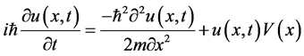(1)

where:

is complex dependent variable;

x is a boundary-value (spatial) independent variable;

t is initial-value independent variable;

is Planck constant;

i is an imaginary complex number.

According to [9] , by letting and normalizing and 2m to unity Equation (1), can be written in the form

(2)

where q is arbitrary parameter.

In subscript notation Equation (2) can be written as

(3)

Replacing the spatial derivative by a second order finite difference approximation in Equation (3) and following [10] , the function, , is replaced by the sum of its real part and its imaginary part in the form

(4)

Substituting Equation (4) into Equation (3), the two equations:

(5a)

or

(5b)

are obtained.

Equating the real and imaginary parts of Equations (5a) and (5b) to zero, the following nonlinear system of PDE

(6a)

(6b)

is obtained.

From Equation (6a) the equations:

(7a)

or

(7b)

are obtained.

From Equation (6b),

(8a)

or

(8b)

are obtained.

Replacing the second order partial derivative in Equation (7b) by the three point central difference approximation and to the replacing the second order partial derivative by its equivalent three point central difference approximation in Equation (8b) where h is the space between the discretized line and n is the number of grids, the following equations are obtained.

(9a)

(9b)

According to [11] , the analytical solution of Equation (3) is

(10)

To analyze as two real functions it is obtained that

(11)

Equations (9a) and (9b) constitute the discretized form of the real and imaginary parts of Equation (3) by the MOL respectively. The real and the imaginary parts of the solution of the Schrodinger equation are independent, identically distributed standard normal random variables with mean 0 and variance 1 [12] . Hence Equation (9a) or (9b) can be chosen for computational purposes. In this paper we shall use Equation (9a) and, for the numerical integration.

3. L-Stable Implicit Trapezoidal-Like Integrator

The trapezoidal-like integrator

(12)

shall be used in the numerical integration, where:

(13a)

(13b)

are the first and second eigenvalues of the discretization matrix respectively; l is the time step; and denotes differentiation with respect to time.

The derivation of the method (12) and the analysis of the order of accuracy are as discussed in [13] .

3.1. Stability Properties of the Method (12)

In this section, we state and prove one lemma and two theorems which relate to the stability property of the method (12) as follows:

3.1.1. Lemma 1

Let and be the eigenvalues of the system of ODE evolved by discretizing the Schrödinger equation by the MOL; and let and. Suppose the following conditions hold:

1) if and

2) if

Then, in Equation (12),.

Proof.

Given that if and if

and.

But and; given.

and.

But

and.

Hence

(13)

All the quantities on the L.H.S. of inequality (13) are positive.

Expanding and rearranging the L.H.S. of (13), we have

. (14)

Dividing inequality (14) through by yields

. (15)

Therefore,

. (16)

Resolving inequality (16) into partial fractions, we have

. (17)

From Equations (17), (13a) and (13b), we have that.

This proves the Lemma 1.

3.1.2. Theorem 1

The numerical integrator (12) is A-stable.

Proof.

Applying the test equation

. (18)

To the method in Equation (12) and from the general linear multistep method.

The Schur’s polynomial is thus given by

(19)

(20)

(21)

By Schur’s condition

(21)

Hence

(23)

But as proved in Lemma 1, hence

The numerical integrator (12) is therefore A-stable.

3.1.3. Theorem 2

The numerical integrator is L-stable.

Substituting the scalar test Equation (18) into Equation (12) yields

(24)

(25)

(26)

Hence

(27)

Substituting for R and S in Equation (27), simplifying and taking the limit by use of L’Hospital’s rule we obtain

(28)

Hence, the proof of the Theorem 2. Thus the integrator (12) is L-stable.

4. Computation of Absolute and Relative Errors

In this section we explain how the absolute and relative errors of the methods shown in the Table 1 and Table 2 were obtained.

4.1. Absolute Errors

The absolute errors of the scheme were computed by the use of the formula:

where the numerical solution at the grid point is and the analytical solution at the same grid point is

4.2. Relative Errors

Relative errors of the method were computed by use of the formula:

where the numerical solution at the grid point is and the analytical solution at the same grid point is

5. Results and Discussion

On the implementation of the L-stable implicit trapezoidal-like integrator for the solution of one-dimensional time dependent Schrödinger equation after discretizing with the MOL, the errors and relative errors of the scheme were computed as shown in Table 1 and Table 2 respectively. The L-stable property of the scheme is supported by the fact that the maximum relative errors at the various discretization levels are not significantly different as shown in Table 3. The performance of the trapezoidal-like integrator compares favorably with the

method of [10] as shown in Table 4. This indicates that the method is considered to give more accurate and stable results at the various spatial discretization levels considered. All computations and plotting of Figure 1 and Figure 2 in this paper were carried out using Maple 15.

References

NOTES

^*Corresponding author.

References

- Becerril, R., Guzman, F.S., Rendon-Romero, A. and Valdez-Alvarodo, S. (2008) Solving the Time Dependent Schröd- inger Equation Using Finite Difference Method. Revista Mexicana de Fisica E, 54, 120-132.
- Jiménez, S., Iorente, M.I.L., Manch, M.A., Peréz-García, M.V. and Vázquez, L. (2003) A Numerical Scheme for the Simulation of Blow-Up of the Nonlinear Schrodinger Equation. Applied Mathematics and Computation, 134, 271-291. http://dx.doi.org/10.1016/S0096-3003(01)00282-X
- Ramos, J.I. and Villatoro, F.R. (1994) The Nonlinear Schrodinger Equation in the Finite Line. Mathematical Computer Modeling, 20, 31-59. http://dx.doi.org/10.1016/0895-7177(94)90030-2
- Zisowsky, A. and Ehrhardt, M. (2008) Discrete Artificial Boundary Condition for Non-Linear Schrodinger Equations. Mathematical and Computer Modeling, 47, 1264-1283. http://dx.doi.org/10.1016/j.mcm.2007.07.007
- Ismail, A.I.N., Karim, F., Roy, G.D. and Meah, M.A. (2007) Numerical Modeling of Tsunami via Method of Lines. World Academy of Science, Engineering and Technology, 1, 341-349.
- Hoz, F. and Vadillo, F. (2008) An Exponential Time Differencing Method for Nonlinear Schrodinger Equation. Computer Physics Communication, 179, 449-456. http://dx.doi.org/10.1016/j.cpc.2008.04.013
- Thron, C. and Watts, J. (2013) A Signal-Processing Interpretation of Quantum Mechanics. The African Review of Physics, 8, 263-270.
- Schiesser, W.E. (1991) Numerical Method of Lines: Integration of Partial Differential Equation. Academic Press Limited, California.
- Schiesser, W.E. and Griffith, G.W. (2009) A Compendium of Partial Differential Equation Model: Method of Lines Analysis with Matlab. Cambridge Universal Press, Cambridge. http://dx.doi.org/10.1017/CBO9780511576270
- Sa’adu, L., Hashim, M.A., Dasuki, K.A. and Sanugi, B. (2012) A Method of Lines Approach in the Numerical Solution of 1-Dimensional Schrӧdinger Equation. Applied Physics Research, 4, 88-93. http://dx.doi.org/10.5539/apr.v4n3p88
- Samrout, Y.M. (2009) New Second and Fourth Order Accurate Numerical Schemes for the Cubic Schrodinger Equation. International Journal of Computer Mathematics, 8, 1625-1651.
- Proakis, J. (2000) Digital Communications. 4th Edition, McGraw-Hill Publishing, New York.
- Fatokun, J.O. and Akpan, I.P. (2013) L-Stable Implicit Trapezoidal-Like Integrators for the Solution of Parabolic Partial Differential Equations on Manifolds. African Journal of Mathematics and Computer Science Research, 6, 183-190.