American Journal of Operations Research
Vol. 3 No. 1 (2013) , Article ID: 27512 , 16 pages DOI:10.4236/ajor.2013.31001
Computational Tools to Support Ethanol Pipeline Network Design Decisions
Production Engineering Program, Federal University of Rio de Janeiro, Rio de Janeiro, Brazil
Email: *gustavodias.po@gmail.com, virgilio@ufrj.br, laura@pep.ufrj.br
Received November 16, 2012; revised December 17, 2012; accepted December 30, 2012
Keywords: Ethanol; Pipelines; Network Design; Mathematical Programming
ABSTRACT
This paper considers the pipeline network design problem (PND) in ethanol transportation, with a view to providing robust and efficient computational tools to assist decision makers in evaluating the technical and economic feasibility of ethanol pipeline network designs. Such tools must be able to address major design decisions and technical characteristics, and estimate network construction and operation costs to any time horizon. The specific context in which the study was conducted was the ethanol industry in São Paulo. Five instances were constructed using pseudo-real data to test the methodologies developed.
1. Introduction
People use networks daily (sometimes unwittingly) in a wide range of contexts. Telephony networks, logistics networks for freight transportation and distribution networks (water, energy) provide services that are essential to modern life and, therefore, must be properly designed to ensure service quality and meet user demands.
Brazil is projected to be both a major producer and supplier of biofuels, particularly biodiesel and ethanol. These fuels are gaining importance on the world stage in view of the environmental, technological and economic impacts caused by global dependence on fossil fuels, particularly oil [1].
However, Brazil’s transport logistics system still rests largely on its highway network, which—although economically competitive—is not safe for transporting fuel, especially in large volumes. A paradigm shift must take place and Operations Research can help in that process.
This study aims to provide robust and efficient computational tools to assist decision makers in evaluating the technical and economic feasibility of ethanol pipeline network designs. Such tools must be able to address major design decisions and technical characteristics, and estimate network construction and operation costs to any time horizon.
The paper is organized as follows: Section 2 presents the context that motivated the research; Section 3 describes the problem under study, characterizing it in technical and theoretical terms; Section 4 presents the optimization approaches taken to solving the problem; Section 5 reports the results and conclusions; and Section 6 offers some final remarks on the study.
2. Context
Current economic growth rates have generated increasing demand for oil. Consequently, market laws exert strong pressure on oil prices, which fluctuate, significantly increasing the cost of living. In parallel with this, the environmental effects of global warming are an issue globally. Pollutant emissions from burning fossil fuels aggravate the phenomenon, drawing criticism and spurring the search for viable alternatives [1]. Technological development has also contributed significantly to this substitution. “Flex-fuel” vehicles have reduced fossil-fuel consumption by offering consumers freedom of choice [2].
Ethanol will play an important role in this process: firstly, because large-scale production costs have been competitive with those of oil since 2004, and secondly, because it is a cleaner energy source [3]. Brazil has become critical in this process, because it has the experience and natural conditions for producing ethanol from sugarcane, and has invested strongly and achieved technological improvements since the start of the Proálcool program [4,5]. Figure 1 shows Brazil’s output by region in crop year 2008/2009 [6].
Brazil is now the world’s second-largest producer [4]. According to the Sugarcane Industry Union, [6], production reached 27.5 million cubic meters in crop year 2008/ 2009, and is increasing each season. Figure 2 shows the trend [6]. However, studies have found that bottlenecks in Brazil’s infrastructure significantly affect fuel logistics, burdening links in the supply chain and raising endproduct prices [7].
This result is worrying given that production is not evenly distributed across Brazil. Though concentrated mostly in the southeast [8], due mainly to different production technologies [3], a logistics network is essential to collecting it at lowest possible cost. Pipelines are a particularly appropriate transport mode for such transfers, as they always attain large volumes (Figure 3). Motivated by this context, this study examines the logistics of fuel. The particular problem addressed is how to design a pipeline network to collect the ethanol produced by a set of regions and route it to a pre-determined destination region. Pipelines were chosen for their high reliability and economic competitiveness [9]. São Paulo State was chosen since it is currently Brazil’s largest ethanol producer [6], thus justifying investments in the sector. Figure 2 illustrates its ouptut.
Designing such networks is a complex task due to the large number of technical and economic requirements to be considered simultaneously. Proper project management is imperative, and projects are commonly divided into conceptual and hierarchically dependent phases that characterize their life cycle [10]. A pipeline project consists of the following stages [9]:
• Planning: early stage of the potential enterprise, where technical, economic and social data are collected to assist feasibility evaluation.
• Conceptual Engineering: identifies project technical and economic feasibility, and sets the basic and detail engineering agenda.
• Basic Engineering: the basic design is developed and detailed to consolidate engineering aspects before any procurement and implementation expenditures are made.
• Implementation: step execution and control. Activities typical of this stage include construction and assembly, commissioning and conditioning.
• Operation and Maintenance; Decommissioning: operation of pipeline is terminated because it is obso lescent, supplanted by other systems or no longer of interest to the owner.
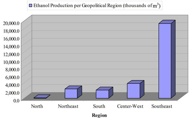
Figure 1. Ethanol production by geopolitical region, 2008/2009 harvest.
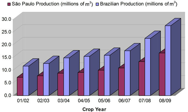
Figure 2. Ethanol production in São Paulo and Brazil.
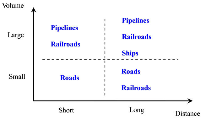
Figure 3. Transport mode comparison matrix.
From an Operations Research viewpoint, meanwhile, Minoux [11] points out that, given a set of nodes, designing a network consists of constructing and/or installing better connections between some pairs of these nodes in compliance with certain operational specifications that govern the application’s behavior. That definition covers the planning and conceptual engineering phases mentioned above, where the main concern is to assess the strategy’s competitiveness, and where the level of technical detail is still low. This study intends to develop computational tools to assist in that endeavor. Silva [12] offers a brief literature review on the PND (and correlated problems). Distribution network designs are frequent, and entail deciding pipeline diameters, pump capacities, reservoir elevation profiles and duct flows, satisfying constraints, ensuring hydraulic energy balance and meeting demand. Such decisions and constraints are handled in an integrated or hierarchical manner, frequently taking topology as given. None address the problem examined here. The most similar, offered by Brimberg et al. [13], consists in designing an optimal pipeline network topology to transport output from oil fields in Gabon by connecting oil wells to a port.
Investment and operating costs tend to be of different orders of magnitude [9]. In the context considered here, however, all information about total project cost is important, since roads historically form the backbone of Brazil’s logistics system [2] and are always an economically competitive alternative. In addition, depending on the time horizon considered, operating costs may influence design decisions. The combinatorial nature of the problem, coupled with the nonlinear equations of fluid dynamics, requires the use of a mixed-integer nonlinear program (MINLP) approach, which is solved via exact and heuristic algorithms.
3. Pipeline Network Design
This section will give an overview of ethnol pipeline network design, indicating the key theoretical and technical characteristics. The problem is formally stated, presenting the technical decisions that are being addressed and the main assumptions. Next a cost analysis is made of pipeline network projects. Finally, the problem is formulated mathematically.
3.1. Fluid Dynamics Considerations
3.1.1. Flows
Flows are caused by the action of a shear stress on a fluid initially at rest. Temporal analysis of a flow allows it to be classified into one of two regimes, namely the transitional (early stage) regime, in which flow velocity, density and temperature parameters at any point vary with time, and the steady-state (perennial stage) regime in which these parameters do not vary with time.
Steady-state flows, in turn, can be classified into two types: laminar, in which fluid particles move along parallel streamlines (paths) without macroscopic interaction between the layers; and turbulent, in which fluid particles move along irregular trajectories with major macroscopic interaction. The dimensionless Reynolds number is used to indicate whether the flow is laminar or turbulent [14].
In ducts, flow may occur under the predominant, but not exclusive, action of two different mechanisms: gravity or a pressure gradient. The main characteristic of flow under gravity, known as open-channel flow, lies in the fact that the fluid flows without completely filling the duct. In the case of flows promoted by a pressure gradient. The ducts are completely filled by the fluid transfer.
Finally, it is possible to characterize two regions in flow along a pipeline: the entrance region, where the velocity field profile is not yet fully developed, and the fully-developed flow region, where the velocity field is the same at any cross-section. The fully-developed region may not exist, but generally, for a pipeline length  and diameter
 , if
, if , it can be assumed that the steady state has been reached.
3.1.2. Energy Issues
Pipeline networks comprise ducts and other components such as valves, bends, fittings, pumps, turbines and tanks. All these elements contribute to system energy dissipation. There are two types of losses, one due to friction between duct walls and the outer layers of the fluid, and the other due to geometric changes in cross-section profiles along the pipeline route. The D’Arcy-Weisbach Equation enables losses to be calculated for incompressible, permanent and fully-developed flows:
 (1)
(1)
where  is the pressure drop along the pipeline whose transferred flow is
  the parameter pi,
  the gravity (m/s2) and
  the friction factor.
Flow machines are mechanical devices capable of extracting energy from fluids (turbines) or adding energy to them (pumps) by dynamic interactions between the device and the fluid [14]. Pumps, in turn, are described mainly by characteristic curves that relate the load provided and the operation flow. Figure 4 exemplifies this. Another important parameter in describing pump energy behavior is the Net Positive Suction Head (NPSH), which relates to cavitation (vapor bubbles inside the device). Commonly, the pressure in the pump’s power section (input) is low and, when this value reaches the vapor pressure of the fluid, a fraction of the liquid evaporates. This phenomenon leads to loss of efficiency and structural damage.
In 1738 Bernoulli formulated the basic equation governing mechanical energy conservation in a fluid flow system. Generalized a few years later, the energy balance for an isothermal, confined, steady and turbulent flow of a viscous fluid that receives work from, and performs work on, flow machines is given by:
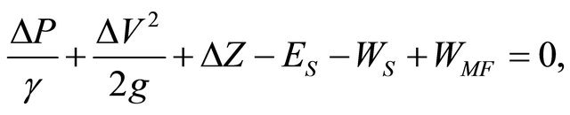 (2)
(2)
where  is the density of the transferred fluid. It represents the sum of pressure (1st term), kinetic (2nd term) and gravitational potential (3rd term) energies in the system, the total power loss
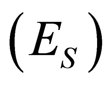 , the work done by the system on its border
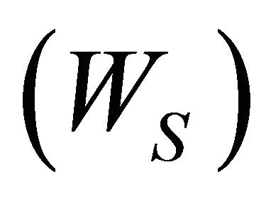 , and the work performed by device B on the system
 .
.
3.1.3. Equipment Selection
Pumps to ensure flows must be selected appropriately not to overestimate or underestimate the equipment’s capacity, thus avoiding unnecessary expense. The system curve is a curve relating energy flow to the load supplied to the fluid, considering the network’s technical and operational features. Consider the system in Figure 5. Substituting Equation (1) into (2), between A and C:
 (3)
(3)
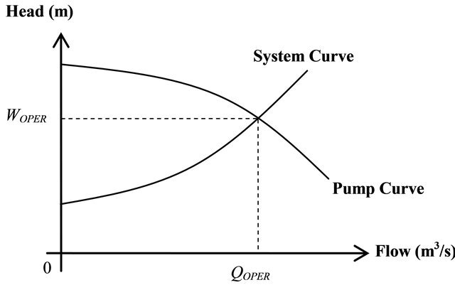
Figure 4. Equipment selection using system and pump curves.
where  and
and  are appropriate parameters. The Equation (3) characterizes the system curve, relating the energy supplied and the flow. This is shown in Figure 4 for a generic set of technical parameters.
System and pump curves are used to choose equipment. Given a system curve and an operating flow , the best-suited pump B to provide the required
  energy is a pump whose characteristic curve intersects the system curve at the desired flow operating point (Figure 4). However, the efficiency curve of the pump should also be considered. Ideally, the operating point should be as close as possible to the highest efficiency point [14]. This latter curve will be disregarded for simplicity.
3.2. General Characteristcs of the PND
Ethanol production is a seasonal activity, and the productive capacity of any region is subject to the conditions necessary for crop development. Such issues make production minimally random in terms of constancy and amount to a given time horizon. Also sugar is produced from sugar cane, and high-demand situations impact ethanol production [15]. Proper treatment of these issues calls for stochastic approaches. Here, however, ethanol output is assumed to be known and not to vary to a given time horizon.
There is no minimum pressure requirement at the end of each section, provided the flow reaches its destination. Hence, pressures will be considered zero at these points. Economic gains also motivate this simplification. Still, assuming that the flows are promoted pressure gradients alone (Section 3.1.1), this hypothesis requires that at least one pumping station be installed at the entrance to each section. This requirement is naturally well conceived, since geographical dimensions require the use of storage tanks, which themselves result in pressure discontinueties.
In an ideal operating regime, storage tanks would be unnecessary in the producer regions, because flow balance would be automatically guaranteed. In practice, in
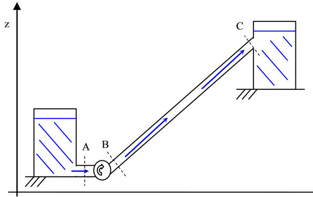
Figure 5. Typical schema of flow within a pipeline.
addition to production inconstancy over time, maintenance system halts are usually necessary, requiring a minimum installed storage capacity in each region. Estimates of such capacities should consider both the randomness of the production and the system downtime schedule, leading again to a stochastic approach. Ideal balance is assumed and also that no storage capacity is required.
The essential nature of services provided by networks requires the system to be able to satisfy design demands even under failure. A redundant network ensures there are at least two distinct paths between any two network nodes. However, this solution requires construction of more pipelines than minimally required to connect all nodes in the network, which in geographically extensive networks, can represent overinvestment. The common solution in such cases is to implement a preventive maintenance policy. It is assumed therefore that the network is designed with no redundance.
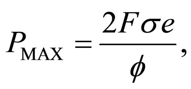
On the other hand, for a given set of technical specifications (diameter, thickness and material output), ducts are certified to withstand a certain maximum operating pressure. That relationship is given by the following equation:
 (4)
(4)
where  is a safety factor [16],
  the circumferential tension in the pipeline,
  the diameter and
  the thickness. The operating pressure is a function of the amount of energy supplied to the system through pumping stations. To prevent limits being exceeded, several stations are placed along sections of the network. For simplicity, however, it is assumed that only one station will be installed in each region. As a result, the maximum operating pressure will occur exactly at the entrance to each section. In a duct with constant flow and speed, zero final pressure and no flow machines, it follows from (1), (2) and (4) that:
 (5)
(5)
where  estimates the maximum value of the flow in the duct.
Route engineering entails certain difficulties. First, it is impossible to build pipelines in straight lines, since there may be impassable terrain between points of interest. Additionally, many slopes may be present in the altitude profile between two regions and this has considerable impact on pump dimensioning. Such issues are to be addressed at data level: the former, when considering distances among the regions, and the latter, using an “equivalent” altitude difference to reflect effects of slopes along routes.
Pump dimensioning is an important issue. This is done to avoid cavitation (Section 3.1.2) by estimating these pumps’ NPSH, which is a function of the height of an equivalent liquid column upstream of the pump. Estimating NPSH, however, would entail estimating the maximum capacity of the tanks upstream of the pump, which would make the mathematical model much more complex. Thus, dimensioning will be done by estimating the downstream energy.
Geographically distributed pipeline networks are subject to temperature variations. This means that fluid property values may change significantly, which may invalidate use of the equations presented in Section 3.1. Thus, flow is assumed to be isothermal. Moreover, it is assumed to occur in a turbulent regime, but in fully developed state, since the distance the flow travels in each network segment is much greater than the pipeline diameter, a necessary condition for such a hypothesis to be true (Section 3.1.1).
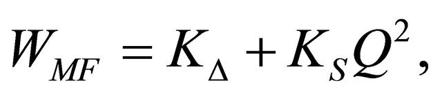
Finally, the flow along the network is not energyconserving (Section 3.1.2). Energy losses are usually offset using pumps in order to ensure system energy balance. Equation (2), used to guarantee this balance in the mathematical model, furnishes an estimate of the energy to be provided to the system at pumps downstream. Losses due to geometric changes will be considered using an estimator for this loss, since there is no way a priori to define the set of components installed. Finally, it is assumed that the flow does not perform work on its surroundings.
3.3. The PND Studied
The problem of designing an ethanol pipeline network, given a set of production regions , a set of associated flows
  and available diameters
 , consists of selecting a subset of links between pairs of these regions to constitute the topology, an associated diameter for each of these connections and, finally, calculating the energy to be introduced into the system to ensure the flow to destination region
 , while minimizing total project cost.
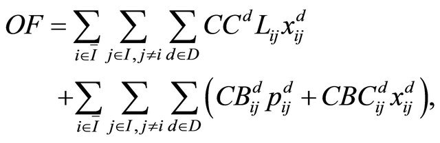
3.4. Cost Analysis
Economically, there are many significant costs in a pipeline project [9]. However it is virtually impossible to deal with them simultaneously, considering the technical complexity involved. One has to select those that represent a significant proportion of project cost, those that can be adequately estimated from the decisions being taken, and those directly influenced by such decisions.
Topology decisions impact on procurement and assembly costs. The same is true of diameters, since different diameters have different prices and are more or less costly to assemble. Pumps are dimensioned (Section 3.1.3) indirectly by calculating from path, length, diameter and flow. Thus, fixed and variable pumping costs are directly influenced by the decisions taken and will be considered in the model.
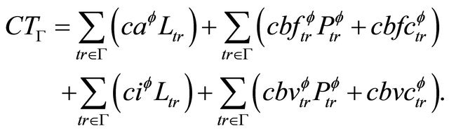
The first three costs are associated with the network construction phase and the last one with the operation phase (to a time horizon ). This can be expressed mathematically as:
 (6)
(6)
where  is total network cost;
  total pipeline procurement cost;
  total pipeline installation cost:
  the total fixed pumping cost; and
  the variable pumping cost to operating time horizon
 .
.  accounts for approximately 17% of total cost [9].
3.4.1. Pipe Procurement
Acquisition cost  can be estimated using the cost per unit mass
  of the material from which they are manufactured. For this, consider the cross-section of sector
  of length
 . Defining
  as the cost of procuring a unit length
  of pipe with internal diameter
 , one obtains:
 (7)
(7)
That is, the unit procurement cost of length of a pipe with diameter  is a function of the cost per unit mass
  of the material
 , the density
 , the thickness of the pipe
  and the diameter
 . Thus:
 (8)
(8)
where  is the set of sectors that constitute the topology. The Equation (8) represents a linear approximation to the total procurement cost.
3.4.2. Network Construction
It is unlikely that an analytical expression exists or can be derived (as in Section 3.4.1) to estimate pipeline installation costs, as installation is a practical task that depends on many factors. However, it may be possible, by empirical analysis of historical data (past projects), to determine approximate, probably non-linear, equations for such costs. However, one can assume that the cost of installing a pipeline sector is directly proportional to its length (the longer the sector length, the greater the amount of resources needed to install it) and depends on the chosen diameter of pipe (handling pipes with different diameters can be more or less costly).
Thus, the cost of installing  is given by:
 (9)
(9)
where  is the cost of installing a unit length of pipewith diameter
 . More complex and realistic cost functions can be used to replace (9), although this introduces nonlinearities into the total project cost function, which would complicate the solution to the problem.
3.4.3. Fixed Pumping
Figure 6 represents the system curve for a sector  of pipeline with diameter
 . For each of the intervals constructed by partitioning the feasible flow space, defined by
  and
and , a pump
  with procurement cost
  is selected (Section 3.1.3). This yields the step cost function represented in Figure 7, for the pressure domain defined by
  and
and .
.
The function obtained takes discrete values that depend on the pressure range sector  is operating in. But selecting a reference pressure for each pressure interval, one can apply a linear regression to obtain the linear pumping cost function shown in Figure 7, defined mathematically by:
 (10)
(10)
where  is the cost of providing a unit of pressure,
  is the fixed cost associated with operating sector
 , and
, and  its operating pressure. The regression must satisfy the condition
  (negative costs
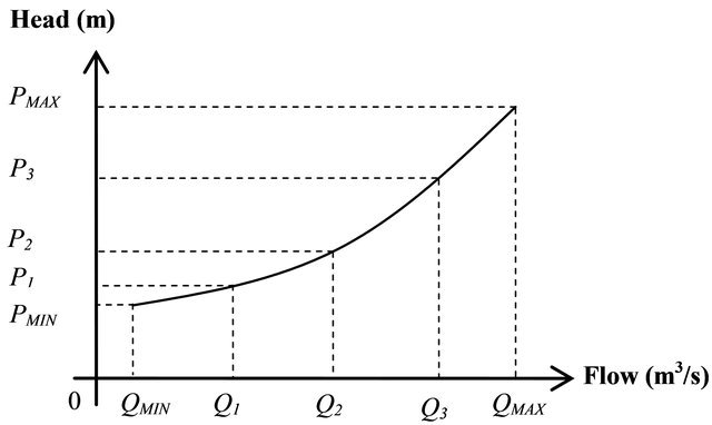
Figure 6. System curve for pipe sector tr with diameter .
.
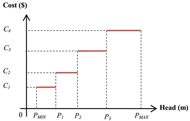
Figure 7. Fixed pumping cost step function (red) and affine function (azul) for sector tr.
for viable pressure values are meaningless). Considering all the sectors that constitute :
:
 (11)
(11)
Regressions for higher degree polynomials can be performed, resulting, however, in the inclusion of nonlinearities in the project cost function.
3.4.4. Variable Pumping
The procedure for estimating the variable pumping cost is the same, except that the costs  associated with the selected pumps represent the cost of operating them to time horizon
 . Thus, the operating cost of
  for
for  can be estimated by:
 (12)
(12)
where  is the cost of providing a unit of pressure in sector
 ,
,  is the fixed cost of operating the sector, and
  the operating pressure. The resulting expression is not time-dependent, but is addressed indirectly in (12). The positivity issue also applies here, as do higher-order regressions.
3.4.5. Total Cost
Substituting (8), (9), (11) and (12) in (6), the overall cost  of network
  may be estimated by equation:
 (13)
(13)
Note that (13) was derived considering only one diameter value , but will be generalized later.
3.5. Mathematical Modeling
The set of producing regions and candidate links can be represented by a complete digraph, where vertices are regions and edges the links between them. Values for distances and inter-region height differences are associated with edges. Similarly, a graph can be associated with the designed network structure. The graph that satisfies the coverage condition for all regions with the fewest connections is a spanning tree (ST) [17], which is adopted as a solution. The formulation by Gavish [18] will be taken as the basis for modeling.
3.5.1. Sets, Indexes and Nomenclature
The set of regions is represented by  and diameters by
 . The reduced set of regions is defined by
 . The indexes
  and
and  and index
  represent the regions and the diameters, respectively. An edge or link
  interconnecting any two vertices is called a sector of the network. For a sector
 , the flow takes place in the direction
 . Accordingly,
  is the initial (input) vertex and
  the final (output) vertex of the sector considered.
3.5.2. Decision Variables
Define binary variable , with value 1 if the sector
  is selected and 0 otherwise. To quantify the flow associated with each sector, we define the nonnegative continuous variable
 . We define the continuous variable
  to quantify the energy supplied in the region
  of a sector
 .
.
3.5.3. Constraints
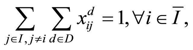
Initially, it must be ensured that all regions will be served by the network. Therefore, except for the destination region, each must have at least one sector through which to dispatch its production. Since the desired topology is a ST, the condition that only one flow exit exist per region shall be forced. Mathematically:
 (14)
(14)
That is, for every region , only one pair
  may be selected. It is important to note that the equation does not restrict the number of sectors ending at any region.
It is necessary to ensure the flow balance in the regions. For every region , the incoming flow from
  at
at , plus its own production, is sent to
 , where
  to avoid cycles. Mathematically:
 (15)
(15)
There is flow in sector  if it is selected, i.e.,
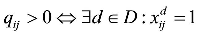 . To ensure that condition, the following constraints can be used:
 (16)
(16)
where:
 (17)
(17)
 (18)
(18)
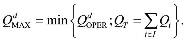
The lower bound  is defined as the lowest production of all regions. The upper bound
  is defined as the lesser value of the maximum flow supported by the pipe or the total output being drained along the network. That is, at no time can any flow traversing the sector
  be below
  or above
 , and flow is zero if the sector is not chosen.
No explicit constraint was introduced to ensure that the solution topology is an ST, or even to ensure flow to destination ; nonetheless, restrictions (14), (15) and (16) together, ensure both conditions [18]. Basically, if the topology has cycles, the balance equations are satisfied only if there is more than one flow exit sector at some of the nodes of the cycle or if there is consumption at any of them.
Finally, to ensure energy balance, the amount of energy that must be provided to compensate for system losses must be estimated. In energy terms, each sector of the network can be viewed as an independent system with its own characteristics (flow, diameter, length, altitude difference etc.). Applying the assumptions of Section 3.2 to (2), it follows for every sector that:
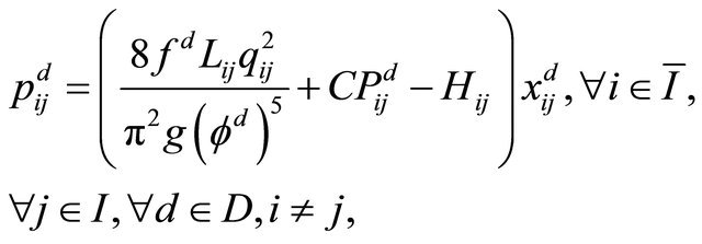 (19)
(19)
where  is the estimated losses due to geometry changes for the sector
 . By hypothesis,
 .
.
So  represents the energy to be provided at
  and not a pressure gradient within
 . Finally, the variable domain constraints:
 (20)
(20)
 (21)
(21)
 (22)
(22)
3.5.4. Objective Function
The Equation (13) will be taken as the objective function. Using the decision variables defined in Section 3.5.2, gives:
 (23)
(23)
which was generalized to consider all diameters in . Note that when
 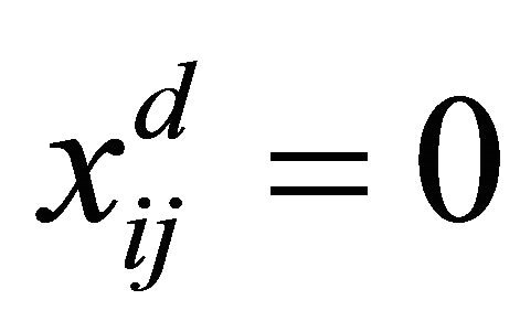 no contribution by any cost related to
  is added to the project total cost.
3.5.5. General
The mathematical programming formulation (MF) of the problem is as follows:
MF: Minimize (23) subject to (14)-(16), (19)-(22).
4. Sollution Approaches
4.1. General Considerations
MF can be manipulated. The  variables appear only in the energy balance constraint (19), domain constraints (22) and objective function (23). The constraint (19) is an equality and, therefore, may be incorporated into the objective function. The variables
  can, in turn, be deleted from the formulation, together with constraints (22). Substituting (19) in (23), gives the new objective function of MF, where
  and
and  are appropriate parameters:
 (24)
(24)
4.2. Heuristic
We consider (24) to develop the algorithm. By evaluating its parameters, three characterizations of a good solution to the problem can be inferred. First, consider the total length in a feasible solution :
:
 (25)
(25)
where . Both portions of cost in (24) are, in some sense, directly proportional to
 . The smaller the total length of the solution network, the lower the cost associated with it. Second, consider
  (Figure 8), where
  is the destination vertex.
Additionally, suppose that  is one of the vertices with highest output among producing regions and that
 , where
  represents the total length of the path connecting vertices
  and
and , and
, and  represents the direct connection between
  and
and . The following expression is computed for
  in (24):
 (26)
(26)
That is, the cost is proportional to the square of the flow in  and the length of the sector. In addition, once flows increase in the direction of the destination, it
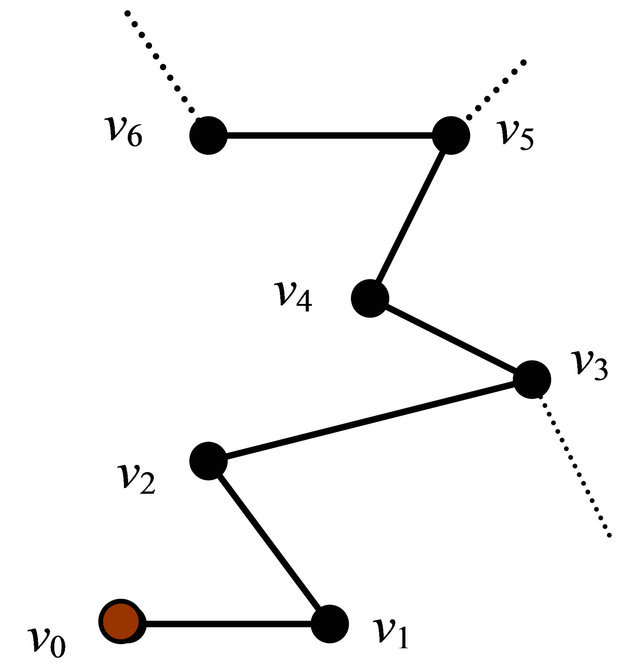
Figure 8. Final part of  with destination
 .
.
can be advantageous to connect  to
to  through the path that minimizes the distance between them (directly, for example) in order to reduce the cost of transportation (operation) between
  and
and , in exchange for building
  additional units of pipe length. The Figure 9 shows the new solution
 .
.
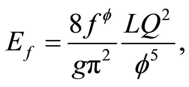
Finally, the cost of  is inversely proportional to the fifth power of the selected diameters and directly proportional to the flows transferred. Since flows increase in the direction of the destination, this increase can be offset by forcing the diameters at least not to decrease in the direction of flow. On the other hand, pipes of larger diameter are more expensive. Thus, it may be beneficial to increase the diameter of sectors with large flows, providing they are as short as possible.
Algorithm Description
Initially, the heuristic PNDH calculates the minimum spanning (MST) tree for the case being solved. This is because the MST is the best estimate in terms of total network length and may be used as initial search point for problems of this nature [19]. The algorithm then defines the flow direction and its value in each sector . The smallest available diameter capable of carrying the flow calculated for each sector is selected. The cost of the initial solution is stored. The algorithm attempts to decrease the distance traveled by large flows and increase the diameter of some sectors, one at a time—in both cases, a predefined number of times. At each trial (path reduction and diameter increase), the new solution is stored if it improves cost.
4.3. Exact
The MF is solved via an exact Outer Approximation algorithm proposed by Duran and Grossmann [20] for MINLP. Although the proposed model does not take into account all the necessary assumptions (linearity of the discrete variables, convexity of the nonlinear functions involving continuous variables and separability on the decision variables) to ensure the convergence of the algorithm to global optima, these global optima were obtained [12].
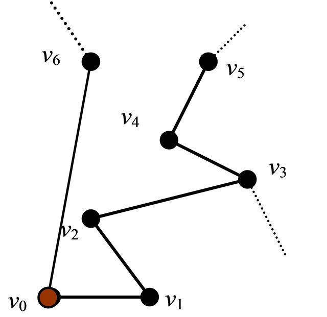
Figure 9. Final part of  with destination
 .
.
5. Computational Experiments
Computational experiments were conducted to test the efficiency and robustness of the model and algorithms. Because it is an original application to the PND problem, the literature on the subject contains no instances; these had first to be built. This section presents the cases constructed, the results obtained with the algorithms and the main conclusions from the analysis of these results.
5.1. Instances
To build instances, the sugar industry of São Paulo was taken as context. In particular, Figure 10 shows the production capacity (millions of cubic meters) and its geographic distribution in 2006 [21]. The regions were named after the largest city in each region.
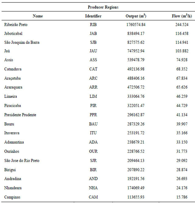
It can be readily seen how decentralized production is and how essential it is to use an appropriately designed and economically competitive logistics network to collect and concentrate production. Table 1 shows numerical values for output from each of the regions in 2006 [21].
Five instances were built, respectively with 4, 8, 12, 16 and 20 producing regions selected from among those listed in Table 1. Only five were built because, technically, a pipeline network designed to connect 20 producing regions can already be considered large. Besides, there was no access to real data.
The distances between regions were determined using the geographic coordinates of the main town. The height differences were calculated directly via the towns’ altitudes. The outputs to be dispatched are listed in Table 1. To determine the associated flow of ethanol, the system was considered to operate three hundred days a year, twenty-four hours a day. The resulting flow rates are listed in Table 1. The idea is to consider network downtime indirectly.
To compose the instances, a set of six possible values for the pair “pipe diameter and thickness” was considered. Four of these pairs were associated with the smallest instance and all of them with the largest one. Table 2 shows the nominal values of the diameters and thicknesses:
Classical empirical equations were used to calculate the friction factors. There are three parameters to be considered in this calculation: diameter, relative roughness [14] and Reynolds Number. The diameters are listed in Table 2. The relative roughness is a characteristic of the pipeline construction material, and the material selected was carbon steel [9]. Reynolds Numbers cannot be calculated as a priori every pipe flow is unkown. Accordingly, an average flow traversing the network was considered for each available diameter.
In all cases, the loss estimator was considered similar
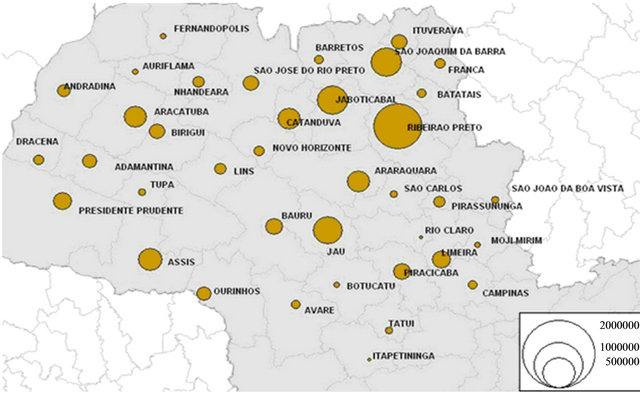
Figure 10. Geographic distribution of ethanol production in São Paulo—2006.
Table 1. Producer regions and associated output in São Paulo—2006.
for every , i.e.,
 . Construction unit costs were determined using Equation (7). The unit cost of carbon steel was obtained in [22]. Since pump commercial prices and real consumption data (
 costs) were not obtained, the methodologies proposed in 3.4.3 and 3.4.4 were not used. Thus, the coefficients of the second portion of (23) were sorted so as at least to respect the percentage given in Section 3.4. Table 3 summarizes the values of technical parameters used in constructing the instances. Table 4 summarizes the characteristics of the instances.
Table 2. Pipe diameter and thickness values considered.
Table 3. Adopted values to technical parameters.

Table 4. Basic description of instances.

5.2. Results
The experiments were performed on an Intel Core 2 Duo 2.66 GHz with 8 GB of RAM. The PNDH heuristic was coded in ANSI C++. The MF was programmed in the commercial software AIMMS [23] and solved with the AOA package available in AIMMS. The OA algorithm problem solvers used were CPLEX 12.1 and CONOPT 3.14 M. The destination region is Campinas.
Table 5 shows the objective function values, PNDH and MF execution times, and a comparative analysis of results in terms of economic gains offered by the solutions. PNDH runtimes were null in all cases. MF produced the best solution for each case, which was obtained in low runtimes, as shown. By comparison, PNDH was able to find two optimal solutions (~0%). The others solutions entail small economic losses ranging from 2% to 6.7%.
We now analyze solutions in non-financial technical terms. Figure 11 represents the optimal design for the case PND_SP_04_04. It is topologically trivial. An interesting fact, however, is the reduction in diameter observed when passing through Limeira. We would expect the same diameter, since flow between Limeira and Campinas is larger. However, (5) suggests that a pipeline’s maximum operating flow is inversely proportional to its length, which is shorter in sector Limeira-Campinas.
The PNDH solution to PND_SP_08_05 is shown in Figure 12. The network is 943.0 km in length and basically concentrates small outputs at Catanduva to be sent to Campinas via Jau. Only Ourinhos pipes directly to Jau, given their proximity. The production routed through Catanduva requires increased diameters on main sectors D12 and D14, successively. Figure 13 shows the MF solution. The network is 984.0 km length (41.0 km longer). Despite the increase, transferring output from Presidente Prudente to Jau via Ourinhos apparently reduces the transport cost (131.0 km shorter) and the construction cost of the Catanduva-Jau sector (from D12 to D10), since flow is decreased. The changes represent a
Table 5. Upper bounds generated by PNDH, optimal solutions obtained by MF, and percentage economic gains.

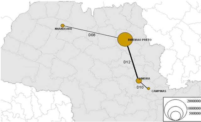
Figure 11. Optimal solution to instance PND_SP_04_04.
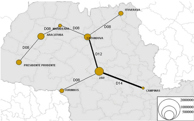
Figure 12. Solution to PND_SP_08_05 by PNDH.
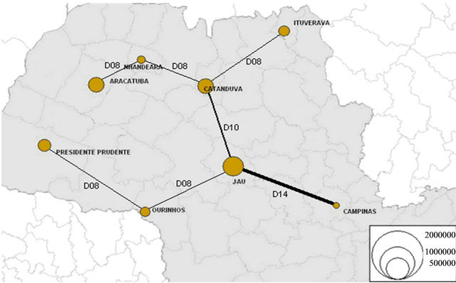
Figure 13. Optimal solution to instance PND_SP_08_05.
1.72% saving in project cost (Table 5).
Figure 14 represents the optimal solution obtained to PND_SP_12_05, with 973.0 km total pipeline length. Interestingly, output from Nhandeara is initially transported to the west, away from Campinas, probably because the output is so small that it is not worthwhile connecting it to Ribeirao Preto or Bauru, 239.0 and 207.0 km away, respectively, even if the segment Adamantina-Assis (128.0 km) were removed, for example, in order to increase Nhandeara’s throughput. Pipe diameter increases significantly at Jau, because it concentrates almost all output even before it arrives at Campinas. At Bauru, on the contrary, pipeline diameter is reduced, probably for reasons of geography.
PNDH built the 1040.0 km solution to PND_SP_16_06, as sketched in Figure 15. Prioritizing the shortest possible pipeline length, Ribeirão Preto was connected to Jaboticabal (54.0 km northwest). Since Ribeirão Preto has the highest output (Table 1), pipeline diameter from Jaboticabal increased significantly (from D12 to D16). There is a diameter reduction at Limeira.
As compared with the optimal design (Figure 16), there is little change when leaving Ribeirão Preto, from which flow now travels 75.0 kilometers to Araraquara. This adds 21.0 km to the network (1061.0 km), reduces the construction costs of the Jaboticabal-Araraquara sector (from D16 to D12) and transport costs of output from Ribeirão Preto. The change represents a 1.17% project cost saving (Table 5). Finally, it is advantageous to transport output from Assis to Araraquara via Presidente Prudente (582.0 km) rather than connecting them directly. Increased production could justify a direct connection.

Figure 14. Optimal solution to instance PND_SP_12_05.
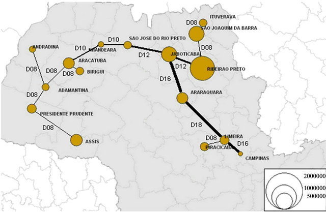
Figure 15. Solution to PND_SP_16_06 by PNDH.
Finally, Figure 17 represents the PNDH solution to PND_SP_20_06 (1361.0 km). Interestingly, Ribeirão Preto was connected to Campinas and not to a closer region (Araraquara or Limeira). This is because connecting it to Araraquara entails increasing diameters all the way to Campinas, thus also increasing the solution cost. Nevertheless, the Ribeirão Preto-Campinas connection does not form part of the optimal solution (Figure 18), since dispatching from Ribeirão Preto to Araraquara is economically favorable. This modification undermines the heuristic topology (Araraquara-Jau), making it necessary to detour flow from Araraquara to Limeira. This modifies pipe diameters in the final portion of the network, reduces the network length to 1282.0 km and represents a 6.7% saving in project cost (Table 5). Pipeline diameter is reduced at Piracicaba.
5.3. Conclusions
These findings emphasize the quality of the solutions built by PNDH (economic losses of less than 6.7% at null computational time cost). This result confirms the potential of the set of characterizations of a good solution. However, the most encouraging results were those generated by the exact algorithm. All except the largest case were solved in very low computational times. Improvement may possible be achieved by inputting information from the heuristic solution to the OA algorithm.
The tools developed to solve the PND addressed here met the expectations of robustness and efficiency and can be used as decision support tools for projects of this nature. Indeed, as the PND relates to a pipeline network whose purpose is to channel fluids to some central location,
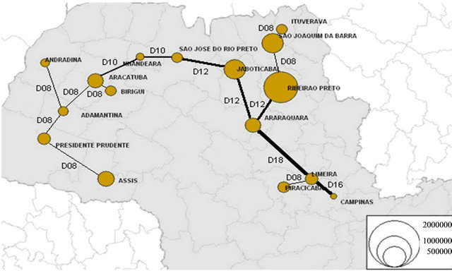
Figure 16. Optimal solution to instance PND_SP_16_06.
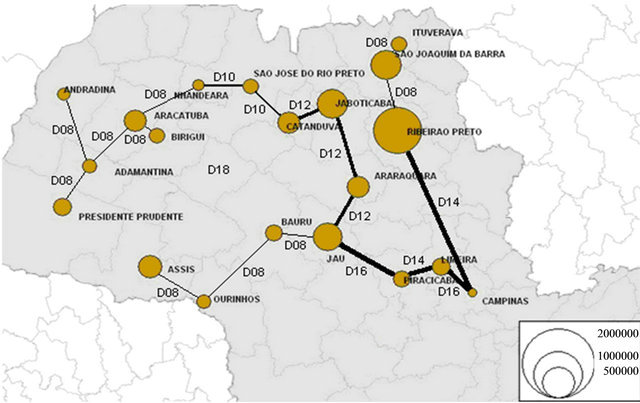
Figure 17. Solution to PND_SP_20_06 by PNDH.
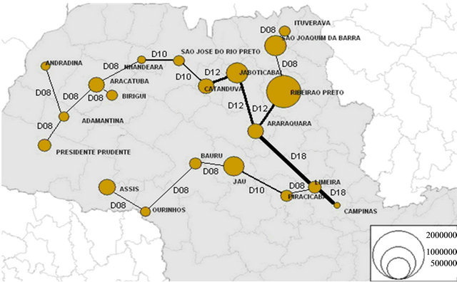
Figure 18. Optimal solution to instance PND_SP_20_06.
and where the main characteristic of the required solution is a topology without cycles and with pressure discontinuities at vertexes, these tools can be used.
6. Final Remarks
6.1. General
In this study, the problem of designing pipeline networks to transport fuel was addressed with a view to developing robust and efficient computational tools able to consider and assess the main design-related technical characteristics and decisions, as well as to estimate the construction cost and the operating cost (to any time horizon), in order to assist decision makers when evaluating the technical and economic feasibility of such projects.
Technical decisions are interdependent. For example: for a given flow rate, the larger the diameter of the duct, the lower the power dissipation. Thus pumps can be smaller and cheaper. However, the larger the diameter, the more expensive the pipe becomes. Conversely, if pipe diameter is diminished in order to reduce construction cost for the same flow rate, power dissipation is higher and thus higher-capacity (and more costly) pumps have to be installed. The larger the network, the harder it is to address these issues.
Accordingly, the combinatorial nature of the problem coupled with non-linear equations governing the flow energy balance, recommended the use of MINL mathematical programming models. To solve the problem, a heuristic algorithm that traces the main features of a technically feasible solution was developed to search for the best possible solutions in terms of cost. The mathematical program was coded in the AIMMS development environment, which provided the necessary optimization tools.
The particular context adopted was the ethanol industry in São Paulo State. The tools developed were tested on five cases built on the basis of output data from around the state. The computational results were extremely satisfactory, since all cases were solved efficiently by the heuristics, and also to global optimality by the exact algorithm, with low execution times, thus confirming the robustness of the approaches adopted.
6.2. Future Work
The most radical paradigm that can be broken is the deterministic approach. The assumption that the supply of ethanol is uncertain to the operating time horizon would probably lead to addressing the time variable directly, in order to design a network that best suits many different possible supply scenarios, as well as to using stochastic mathematical programs.
Technically, there are many options. Allocation of more than one diameter per sector of pipeline in the network may be considered. Pressure loss will be calculated as the sum of the losses in each of the sub-sections with different diameters. The energy balance equation should consider the different kinetic energy in the sectors, since different cross-sections produce different flow velocities for the same flow rate.
Another variant might consider finite storage capacities in the regions, to be decided in view of the related cost. This capacity is influenced by the stochasticity of production and the NPSHR pump parameter. If only the latter is considered, a stochastic approach to the problem can be avoided by estimating the minimum storage capacity of each region.
Finally, it would be useful to determine the number and location of pumps needed to power the system. Motivations to treat this decision are that it may not be possible to provide all the power necessary in each region by using one single station (technical limitation) and that, since pipes have maximum pressure tolerances, it may be necessary to distribute the energy supplied so that theses limits are observed.
7. Ackowledgements
The authors would like to thank the Agência Nacional do Petróleo, Gás Natural e Biocombustíveis (ANP) for financial support provided under grant PRH-ANP-21.
REFERENCES
- J. Goldemberg, “Ethanol for a Sustainable Energy Future,” Science, Vol. 315, No. 5813, 2007, pp. 808-810. doi:10.1126/science.1137013
- H. Pacini and S. Silveira, “Consumer Choice between Ethanol and Gasoline: Lessons from Brazil and Sweden,” Energy Policy, Vol. 39, No. 11, 2010, pp. 6936-6942. doi:10.1016/j.enpol.2010.09.024
- R. G. Compeán and K. R. Polenske, “Antagonistic Bioenergies: Technological Divergence of the Ethanol Industry in Brazil,” Energy Policy, Vol. 39, No. 11, 2011, pp. 6951-6961. doi:10.1016/j.enpol.2010.11.017
- A. Hira and L. G. Oliveira, “No Substitute for Oil? How Brazil Developed Its Ethanol Industry,” Energy Policy, Vol. 37, No. 6, 2009, pp. 2450-2456. doi:10.1016/j.enpol.2009.02.037
- A. T. Furtado, M. I. G. Scandiffio and L. A. B. Cortez, “The Brazilian Sugarcane Innovation System,” Energy Policy, Vol. 39, No. 1, 2010, pp. 156-166. doi:10.1016/j.enpol.2010.09.023
- União da Indústria de Cana de Açucar, “Dados e Cota- ções-Estatísticas,” 2009. http://www.unica.com.br/dadosCotacao/estatistica
- Centro de Estudos Logísticos e Instituto Brasileiro de Petróleo, Gás e Biocombstíveis, “Planejamento Integrado do Sistema Logístico de Distribuição de Combustíveis,” 2008. www.ibp.org.br
- L. C. Freitas and S. Kaneko, “Ethanol Demand in Brazil: Regional Approach,” Energy Policy, Vol. 39, No. 5, 2011, pp. 2289-2298. doi:10.1016/j.enpol.2011.01.039
- J. L. F. Freire, “Engenharia de Dutos,” ABCM, Rio de Janeiro, 2009.
- Project Management Institute, “Um Guia do Conjunto de Conhecimentos em Gerenciamento de Projetos (Guia PMBOK®),” 3rd Edition, PMI Publications, Newtown Square, 2004.
- M. Minoux, “Network Synthesis and Optimum Network Design Problems: Models, Solution Methods and Applications,” Networks, Vol. 19, No. 3, 1989, pp. 313-360. doi:10.1002/net.3230190305
- G. D. Silva, “Abordagens Heurísticas e Exatas para o Problema de Projeto de Redes de Dutos,” M.Sc. Thesis, COPPE/UFRJ, Rio de Janeiro, 2009.
- J. Brimberg, P. Hansen and K. Lih, “An Oil Pipeline Design Problem,” Operations Research, Vol. 51, No. 2, 2003, pp. 228-239. doi:10.1287/opre.51.2.228.12786
- B. Munson, D. F. Young and T. H. Okiishi, “Fundamentos da Mecânica dos Fluidos,” 4th Edition, Edgard Blücher, São Paulo, 2004.
- J. R. Moreira and J. Goldemberg, “The Alcohol Program,” Energy Policy, Vol. 27, No. 4, 1999, pp. 229-245. doi:10.1016/S0301-4215(99)00005-1
- B. C. Forlano and R. Maclain, “Facilities Piping,” Paragon Engineering Services, Houston, 1991.
- F. Harary, “Graphs Theory,” Addison-Wesley, Reading, 1969.
- B. Gavish, “Topological Design of Centralized Computer Networks—Formulations and Algorithms,” Networks, Vol. 12, No. 4, 1982, pp. 355-377. doi:10.1002/net.3230120402
- F. Rothlauf, “On Optimal Solutions for the Optimal Communication Spanning Tree Problem,” Operations Research, Vol. 57, No. 2, 2009, pp. 413-425. doi:10.1287/opre.1080.0592
- M. A. Duran and I. E. Grossmann, “An Outer-Approximation Algorithm for a Class of Mixed-Integer Nonlinear Programs,” Mathematical Programming, Vol. 36, No. 3, 1986, pp. 307-339. doi:10.1007/BF02592064
- L. N. S. M. Dória, “Construção e Entendimento dos Cenários dos Mercados Interno e Externo do Álcool no Brasil (2006-2015),” Final paper on course in Operation Management in Oil Exploration and Production, Polytechnic School, Rio de Janeiro, 2007.
- MEPS LTD, “MEPS—World Carbon Steel Prices—With Individual Product Forecasts,” 2009. http://www.meps.co.uk/World%20Carbon%20Price.htm
- M. Roelofs and J. Bisschop, “AIMMS User’s Guide,” Paragon Decision Technology B.V., 2011. http://www.aimms.com/downloads/manuals/user-s-guide
NOTES
*Corresponding author.