American Journal of Operations Research
Vol. 2 No. 4 (2012) , Article ID: 25138 , 14 pages DOI:10.4236/ajor.2012.24054
Conditional Lot Splitting to Avoid Setups While Reducing Flow Time
1Department of Management, Georgia Southern University, Statesboro, USA
2US Air Force Academy, Colorado Springs, USA
3Department of Marketing and Logistics, Georgia Southern University, Statesboro, USA
Email: jsimons@georgiasouthern.edu
Received October 2, 2012; revised November 5, 2012; accepted November 12, 2012
Keywords: Lot Splitting; Scheduling; Setups; Shop Floor Control; Simulation
ABSTRACT
Previous research has clearly and consistently shown that flow time advantages accrue from splitting production lots into smaller transfer batches or sub-lots. Less extensively discussed, and certainly undesired, is the fact that lot splitting may dramatically increase the number of setups required, making it impractical in some settings. This paper describes and demonstrates a primary cause of these “extra” setups. It then proposes and evaluates decision rules which selectively invoke lot splitting in an attempt to avoid extra setups. For the closed job shop environment tested, our results indicate that conditional logic can achieve a substantial portion of lot splitting’s flow time improvement while avoiding the vast majority of the additional setups which would be caused by previously tested lot splitting schemes.
1. Introduction
Many of the jobs customers submit to production facilities consist of requisitions for multiple units, thereby requiring repetitive processing of the units within the job at each operation. While the term process batch refers to the total number of units processed between setups, the term transfer batch has been used to refer to the interoperation movement of portions of a job [1]. Although the size of a particular job may determine the size of the process batch, managers could choose to use a smaller size for transfer batches. Lot splitting refers to a management decision to break down a job into more than one smaller lot or transfer batch.
The reason lot splitting is theoretically advantageous is that the use of smaller lots enables downstream operations to begin sooner. When the first lot of a job proceeds to a subsequent operation, it becomes possible to have more than one operation accomplished on (different portions of) the same job at the same time. In a time when production in small lots has become widely desirable, lot splitting offers the potential to achieve small batch advantages in industries where customers still order in large quantities.
Goldratt and Fox [1] have advocated that transfer batch size should be less than process batch size. This is, in essence, a call for lot splitting. Similarly, just-in-time (JIT) systems seek the minimization of inventory, partly through the use of small transfer batches. If lot splitting is such an excellent idea, why isn’t it universally used? The obvious answer is that there are meaningful costs associated with it. One such cost is additional complexity. However, widely available automated planning and control systems can mitigate this liability. Lot splitting may also increase internal material handling efforts and/or costs because it will increase the number of batches which require movement as well as the frequency with which they must be moved.
However, the significant cost on which this research focuses is the incurrence of additional setups. While small transfer batches enable downstream processing to begin sooner, different lots of the same job might become separated, thereby necessitating “extra” setups. For example, if lot A1 and A2 (both of which are part of job A) become separated, lot B1 (part of job B) might be processed at a particular resource after lot A1 but before lot A2. As a result, the setup necessary for job A might have to be accomplished twice. The general purpose of the present research is to help isolate the factors which lead to these extra setups and identify ways in which lot splitting may be modified to avoid them.
2. Prior Research
Expanding on the review provided by Smunt et al. [2], we have listed some of the more relevant prior research in Table 1. The table suggests something of an evolution in the research. The studies in the first section provided a basis for better understanding how lot size relates to flow time. The studies in the second section sought to apply this relationship in the form of lot splitting to improve flow time in flowshops. The last two sections show efforts to examine lot splitting in environments with greater complexity.
The studies cited in the first section of the table dealt generally with the relationship between lot sizes and job flow times, showing the potential benefits of smaller lot sizes. In particular, Karmarkar, Kekre, and Kekre [3] demonstrated that flow time is a U-shaped function of lot size. As lot sizes begin to shrink, flow times are reduced because some units of a job are able to begin processing at a later machine before other units are finished at the earlier machine (This is sometimes called operations overlapping). Studies have employed various algorithms to examine the relationship between lot sizes and flow times, including the genetic algorithm [4,5] and mixed integer programming [6]. In addition to lot sizes, flow times are also influenced by allocation of work to machines based on processing rate [7]. However, as lots become smaller, the number of setups also increases and at some point the additional setup time overtakes the savings from overlapping, so that flow times begin to increase [8].
The studies shown in the second section dealt more specifically with the possibility of splitting jobs into smaller transfer batches to improve flow times in multistage production systems. The analytical nature of much of this work necessitated its restriction to flow shops with deterministic conditions, such as constant demand and identical machine production rates. The focus of these studies was mostly on determining the best lot sizes. Kropp and Smunt [9] found that heuristic approaches were able to perform nearly as well as optimal ones. Their results showed that equal lot sizes worked well when setup times were small, but that a small “flag” sublot was beneficial when setup times were larger. When setup times cannot be omitted, equal-sized sublots provide better benefits than unequal-sized sublots [10].
The studies in the third section of the table considered the more variable job shop context with stochastic arrivals and processing times. While Wagner and Ragatz [11] studied an open job shop, the other researchers considered various closed job shop cases. Hancock [12] allowed a one-time split of each job into two equal batches at some point after the initial operation in its routing and observed good performance over a range of conditions. Liu [13] studied a job-shop environment with customer order scheduling, using a genetic algorithm to determine the optimal combination of the number of sub jobs of each job and the size of each sub job. In addition to number and size of subjobs, the study by Martin [14] also considered the interleaving of sublots from different jobs in the processing sequence demonstrating significant reductions in makespan. When the size of sublots is held consistent, there is a tradeoff between minimizing makespan and flowtimes. Focusing on minimizing one objective causes significant losses in performance in the objective that was not optimized [15]. The work by Smunt et al. [2] is particularly noteworthy for two primary reasons. First, they examined a broad range of shop conditions. Second, they emphasized the role of variability in arrivals and processing times. These characteristics would seem to make their results more generalizable to environments typically found in practice. Overall, Smunt et al. found that the number of lot splits was more important than the exact form of splitting, although a small initial split (a “flag” lot) proved beneficial in some circumstances.
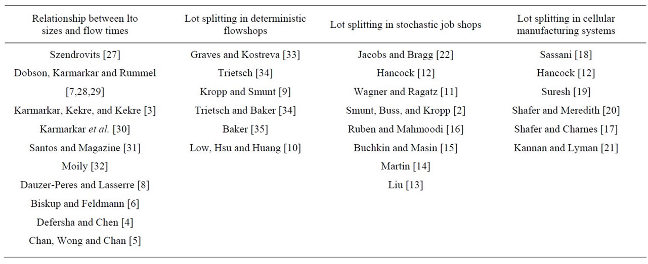
Table 1. Prior studies on lot sizing and splitting.
Ruben and Mahmoodi [16] looked at the effects of lot splitting in unbalanced production systems, i.e. systems where processing times vary across a job’s routing. They considered two specific system structures, each of which contained a single bottleneck. They showed that it makes sense to use different splitting logic at the bottleneck than is used elsewhere in the system. However, it is not clear whether this result can be generalized to other job shops, in which congestion may be a more situational result of dynamic combinations of job requirements and machine availability.
Lot splitting has also been studied in the context of cellular manufacturing (CM) systems. One of the great advantages of CM is that when the machines required to process a family of parts are dedicated and grouped together, both transfer and setup times may be significantly reduced. Shorter setups make it more feasible to employ policies which increase the number of setups. Consequently, lot splitting is even more viable in CM than in functional (job shop) layouts [17].
Sassani [18] found that lot splitting in a Group Technology system is effective when there is only a small setup time penalty and that the setup penalty increases with the number of splits. Although he found results to be situational, he did not specify the variability of processing times within cells. Similarly, Shafer and Charnes [17] found that cellular manufacturing (CM) is superior to a functional layout, provided that operations are overlapped (i.e. lot splitting is used) and setups are reduced. Suresh’s [19] results also indicated that setup reductions must be sufficiently substantial to offset the partitioning effect of converting job shops to cellular manufacturing. Shafer and Meredith [20] found that the benefits of overlapping in CM increased with the required number of machines, batch size, and processing time per part. However, like Ruben and Mahmoodi [16], they found that when bottleneck machines exist, their longer queues limit the benefits of operations overlapping.
Kannan and Lyman [21] specifically acknowledged the tradeoff between flow time improvements due to lot splitting and the additional setups incurred. Their results for a single cell showed that group (family-based) scheduling effectively complements lot splitting. Group scheduling avoids additional setups by giving priority to jobs in a machine’s queue which are similar to the job just completed. This idea was first demonstrated by Jacobs and Bragg [22] in the job shop context, where it was referred to as “repetitive lots”.
In summary, prior research has shown that by taking advantage of the general relationship between lot size and flow times, lot splitting may significantly reduce flow times in a variety of environments. However, splitting one job into several lots is likely to increase the number of setups required. Two approaches have been shown to help reduce the setup impact on flow times. The first is the use of CM. By grouping required machines together, CM may reduce the time per setup so that an increase in the number of setups has less of an impact. But in functional layouts (i.e. job shops) and in CM cases where the time per setup is not negligible, group sequencing rules (e.g. repetitive lots) have been suggested to help reduce the number of setups which must be accomplished.
The prior studies also make it clear that the extent to which lot splitting improves flow times is situational. Although two studies considered a single bottleneck, none of these studies varied the processing time means across stations according to the type of part being produced. In general, the previous research has not dwelt on the question of what factors lead to the increase in setups when lot splitting is used.
3. Research Objectives
While the prior research has acknowledged that lot splitting will increase the number of setups, they have primarily considered this increase in terms of its impact on flow times. As long as the flow time improvements due to lot splitting offset the increased time required for setups, the overall benefit has been perceived as positive.
However, setup includes activities such as tearing down the setup from the previous batch, cleaning the parts to be processed, finding the necessary tools for the new setup, getting and studying the job specifications, adjusting equipment, clamping parts, conducting initial runs, and making adjustments [23,24]. Aside from their impact on flow times, these activities incur personnel, equipment, and raw material costs. These impacts are considered so severe in some settings that jobs are actually delayed to await similar types of jobs in order to avoid setups by forming even larger batches (See pages 288-296 in Hopp and Spearman [25] for an excellent discussion of batching logic). Therefore, in this research, we consider the number of setups to be an important performance measure in its own right.
The prior research also showed that the effects of lot splitting depend on a variety of factors, including the shop’s flow configuration. Therefore, we chose to study a dynamic, stochastic job shop configuration, one of the more problematic scenarios. While other studies have modeled variability within work centers, they have been limited in the extent to which they manipulated the variability across work centers. Our perspective is that if the processing time per part at a particular work center is stochastic, there is no reason to assume the mean times at different work centers will be the same, nor that this source of variability will be limited to a single work station for all job types.
Although much research has been done on lot splitting, the fundamental question addressed so far has been whether lot splitting is good or bad, given various schemes for determining the number and size of sub-lots. The implicit assumption has been that lot splitting is a take-it-orleave-it proposition. This research deviated from that assumption by seeking to show that lot splitting within a specific setting may be sometimes good and sometimes bad. We wished to explore characteristics which determine when each is true and suggest ways in which we could use lot splitting in a job’s routing only when it is most helpful.
Therefore, the present research sought to increase our collective knowledge by helping to better understand when and why lot splitting incurs extra setups. We also demonstrate the extent to which additional setups may be incurred in more variable settings, even when repetitive lots sequencing is employed. Lastly, we use our understanding of the causes of additional setups to better avoid them when lot splitting is used to reduce flow times.
4. Additional Setups Due to Lot Splitting
The purpose of this section is to establish insight concerning when additional setups are likely to be incurred. This information will serve as the foundation for the experiment which is subsequently described.
4.1. Causal Factors
Even when repetitive lots sequencing [22] is used, various factors may cause lots of the same job to become separated. For example, it would seem likely that separation could occur when the mean processing times vary across different operations. Consider the following two cases involving a job which has been split into two lots of five units each for processing at two operations.
In Figure 1, the processing time at the first operation is smaller than the processing time at the second operation. In this case, the additional time required to process units at the second operation permits the units contained in the second lot to enter the second operation’s queue and be ready when the first lot is complete.
By contrast, in Figure 2, the first operation’s processing time is greater than that of the second operation. As a result, the first lot may be complete at the second operation before the second lot is done at the first operation. During the resulting time lag, a lot from a different job may arrive at the second operation and begin processing. Unless this new job is delayed while the affected resource is held idle, a new setup will later be required to process the second lot of the original job. Either way, productive time is lost.
Other factors might also precipitate the separation of a job’s lots. For example, the longer the queue at a downstream operation, the more time the second and subsequent lots of a job would have to catch up. Therefore, short queues might increase the likelihood of additional setups due to separation. In addition to its length, the contents of a queue may affect the likelihood of extra setups. Specifically, the probability that a straggling lot
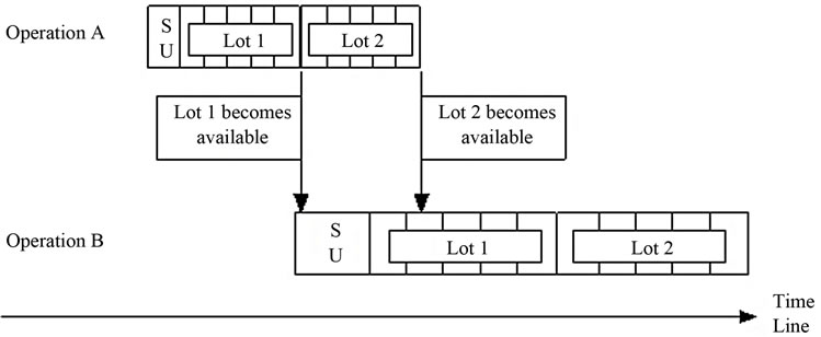
Figure 1. Split lots (smaller time per part on earlier operation).
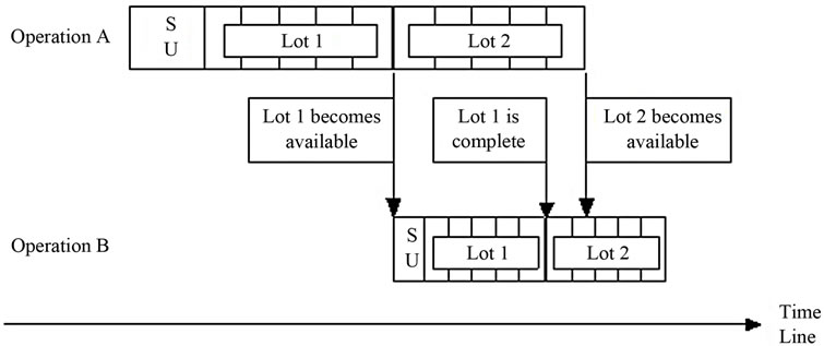
Figure 2. Split lots (smaller time per part on latter operation).
will generate an extra setup should be reduced by the presence of other lots requiring the same setup in its next queue. However, these factors would seem to be lesser since they would be modulated by the extent to which the processing time differential described previously is present.
When these factors are operative (i.e. shorter processing time, shorter queue, or an absence of similar jobs at a job’s next operation), lot splitting schemes would seem particularly prone to increase the number of setups. Any of these circumstances are likely to occur when processing times are stochastic. However, when the processing time distributions are identical at each station, which has been true in most of the models used in prior research, these conditions will occur only randomly and sporadically. By contrast, we postulate that when this phenomenon occurs systematically, e.g. due to a difference in the stochastic distributions (or means) across stations, its effect may be quite pronounced. However, with the exception of single bottlenecks, this factor has not been studied in previous research
4.2. Setup Avoidance through Timing
Although the basic idea of lot splitting is simple, there are actually several decisions involved. Previous research has focused primarily on the questions of the number of splits to be made and the size of the lots.
(Note that the number of splits does not necessarily determine the lot size, since equal-sized lots is only one of many possible alternatives.) However, another potential question is when or where lots should be split. The typical assumption to date has been that jobs will be split into lots upon arrival to the system and will be processed as individual lots until re-assimilated after all processing is complete.
It is appropriate, therefore, to ask whether the advantages of lot splitting can be retained without the disadvantages by manipulating the timing of lot splitting. Since the causal factors discussed in this section are sometimes, but not always present, we suggest the possibility of selectively applying lot splitting as a job progresses through the production system. In other words, there are some points in a job’s routing where it is advantageous to split lots and others where it is not. Using the example presented previously, lot splitting seems desirable in Case 1, but not Case 2.
We suggest that the approach used by Hancock [12] worked well because it manipulated the timing of the lot splitting decision, albeit on a very limited basis. In the case of static, forward scheduling, Hancock was able to avoid the additional setups which unconditional lot splitting would have generated by defaulting to not splitting lots and doing so only when it was both necessary and possible to avoid a job being late. We decided to extend this logic to the dynamic case by splitting and “un-splitting” (i.e. re-joining) a job’s lots as it proceeds through its routing, to take advantage of the conditions encountered.
To invoke lot splitting based on the conditions present at each decision point, we created what we called trigger rules. We used this term because the rules trigger the splitting or rejoining of a job’s lots. Such logic would not be complicated to implement in practice and might well be worth the effort. The specific rules we evaluated are described later in the next section.
5. Research Methodology
The following four subsections describe how the present research was conducted. The first subsection presents the scenario we modeled, based on a foundation provided by prior researchers. We then describe how we modified the basic model to reflect the inequality of process time means described in the preceding section. The third subsection describes the specific conditional logic we tested to see whether we could gain the benefit of lot splitting (improved flow time) without its disadvantage (increased setups). Finally, we specify the remaining details of the data we used and analyzed.
The basic scenario used for the present research was similar to the job shop models studied by Jacobs and Bragg [22] and Smunt et al. [2]. As shown in Figure 3, the shop contained 10 departments, each of which operated a single machine. The shop randomly received orders for 10 different types of jobs. Each job required processing in five of the shop’s departments, with the job type determining which five departments. Every job of the same type followed the same routing, but different job types had different routings. The routings were distributed in such a way that the loads on the different departments were approximately equal.
As jobs arrived at the shop, they were split into lots (described later) if applicable and immediately released to the first required operation. Consistent with prior research, the queue discipline used in each department was “repetitive lots.” According to the logic of repetitive lots, each time a lot completes processing the highest priority is given to other lots in the queue of the same job type.
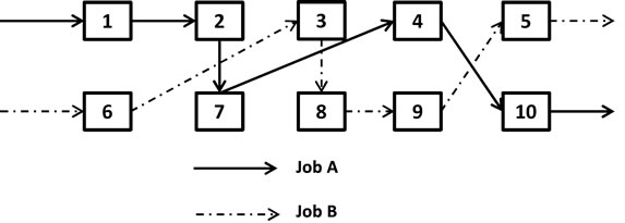
Figure 3. Ten station job-shop (adapted from Smunt et al. [2]).
(Note that these lots may be either other lots of the same job or simply different jobs of the same type.) FIFO was used to break ties and was also the rule used to select the next lot to be processed when the queue did not contain a lot of the same type. By giving preference to lots of the same type, repetitive lots logic obviously seeks to avoid setups.
Setup time can be a source of great variation in the time a job is in the shop. It can vary based on job characteristics, such as the physical dimensions of the unit to be processed. It can also vary based on machine characteristics, such as complexity of the operation to be performed on that machine. A third source of variation is randomness. However, the purpose of this research was not to investigate the impact of variation in setup time, but rather the impact of job splitting. Therefore, setup time was modeled as a multiple of the number of units in an average job, the average processing time per unit on the next machine, and a “setup factor”.
The performance of each scheme was evaluated with respect to three performance measures. The first two, mean flow time (FLOW) and the standard deviation of flow time (SDFLOW), were the primary measures considered by Smunt et al. and seem to be good indicators of customer service (e.g. short response times and consistency). While Ruben and Mahmoodi [16] calculated flow time in terms of individual batches (i.e. transfer batches or sub-lots), we based our calculation on the completion of complete customer jobs, as was done by Smunt et al. [2] and Wagner and Ragatz [11]. In addition, we counted the number of setups per job (NUMSETS) accomplished under each treatment. Although lot splitting has the potential to increase the number of setups required, we wanted to learn the extent to which additional setups were actually occurring rather than simply assuming that they were responsible for observed differences in flow times.
5.1. Equality of Process Mean Times
One of our objectives was to better understand the causes of additional setups. Based on the rationale presented earlier in this paper, we chose to assess the degradation in performance caused by differences among the mean flow times at different stations. Specifically, we wanted to model the effect of the situation where different job types have different processing time distributions at different machines.
To achieve this effect, we produced two sets of runs. The first (M-EQ) used equal mean processing times (0.55 time units per item) at all stations. The second (M-HL) adjusted the processing times for each job type on each machine in such a way that approximately half of the operation times were twice as long as the others. To avoid the potentially confounding effect of a difference in machine loads, we distributed the high and low processing times so that the total loads on the different machines remained approximately equal. Table 2 shows the routing we used for each job type, as well as the mean processing time for each operation.
5.2. Trigger Rules
In previous research, jobs were split into lots upon arrival to the shop and remained split at all operations. We named this benchmark trigger rule T-ALL. (The number and sizes of the split lots are discussed in the next section.) As stated previously, we wished to consider alternate rules in which the decision of whether or not to split a job into smaller lots would be based on one or more conditions having been met. (This research included only the extremes of complete splitting and full reconstitution, and further research would be needed to consider partial reconstitution of jobs.) We tested four conditional trigger rules.
According to trigger rule T-PT, a job was split into
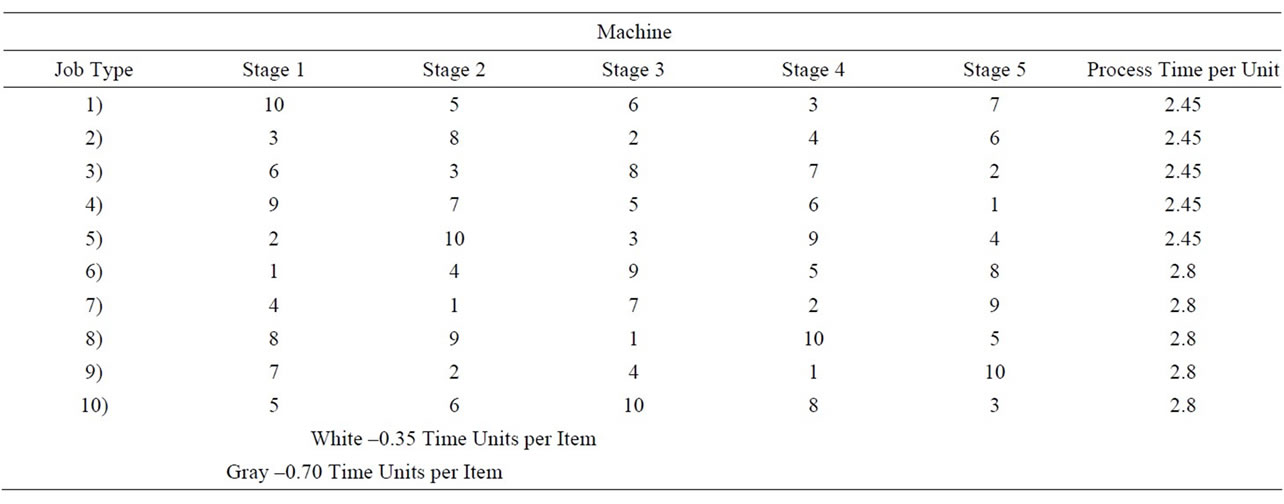
Table 2. Job routings and processing times.
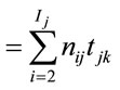
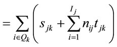
smaller lots only when the mean (per unit) processing time at the next operation was greater than the mean at the current operation, i.e. when tjk + 1 > tjk, where tjk is defined as the processing time of job j on operation k. The idea of T-PT is to use lot splitting in cases such as those represented by Figure 1, but not those represented by Figure 2. A second conditional rule, T-QR, invoked job splitting only when the queue at the next operation downstream contained enough work to lead to the reasonable expectation that the current job would be completed before the next queue empties. That is, if there was enough work in the next queue to occupy that machine using expected processing times until after the current job was expected to be done on the current machine, the job was split. Otherwise, the job was kept together so it would not be separated at the next machine. The following notation defines the rule more specifically.
sjk = setup time for job j on operation k Ij = number of lots in job j nij = number of units in the ith lot of job j Qk = {j: job j is in the queue awaiting operation k}
RPTjk = remaining expected processing time for job j on operation k
QTk = expected setup and process time for work in the queue of operation k
QRjk = queue ratio for job j being processed on operation k
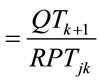
Note that QRjk > 1 suggests we would expect to have time to finish the remaining lots on the current operation before the queue would be emptied on the next operation. Pilot testing indicated that this rule was relatively insensitive to the range of values used as a threshold. The results reported later were obtained by splitting lots when QRjk > 1.
A third conditional rule, T-JT, simply allowed job splitting anytime the downstream queue (Qk) contained a job of the same type as the one being considered for splitting. The idea was that by splitting in this circumstance, we could release the first lot (transfer batch) sooner and perhaps take advantage of the setup which would be generated by the job of the same type in the downstream queue.
The fourth conditional rule, T-PQJ, was a logical union of the first three conditional rules. It caused a job to be split if any of the three conditions called for by T-PT, T-QR, or T-JT was met. Although the most complex of the conditional rules, this rule might have been anticipated to be the most opportunistic in taking advantages of circumstances amenable to lot splitting.
The conditional trigger rules enabled a job to be split into lots at some operations but not others. To achieve this they needed to cause a job’s separate lots to re-join each other when necessary. We used the following logic to facilitate this process. When a job arrived at the shop, it was split into lots according to whatever lot splitting form was in effect. The lots were immediately released for processing at the first operation. As the job’s first lot completed processing at an operation, its routing was checked to determine whether lot splitting was desired at the next operation. If so, the lot was immediately released to the next operation. If not, the lot was held at the output side of the current operation until the remaining lots of the job were also finished processing. (This enabled previously separated lots to re-join each other.) At that time, all lots of the job were released to the next operation.
We reasoned that such policies would be simple to implement in practice. For example, T-PT does not require precise advance knowledge of processing times; instead, it is only necessary to know whether or not the subsequent operation takes longer per unit. Similarly, the required action (if this condition is met) is not difficult to communicate or implement. It is only necessary to treat the entire job as a transfer batch and not initiate delivery to the next queue until the rest of the job is done.
5.3. Other Variables
Smunt et al. [2] considered several lot splitting rules. We chose to consider three of these. RL0 does not split a job into lots at all. This served as our baseline rule, since its performance was needed to determine whether lot splitting improved performance at all. We also applied two of the best-performing of the rules evaluated by Smunt et al. RL3E splits each job into three equal lots. RL4F uses three equal-sized lots preceded by a fourth lot consisting of a single unit. By making this initial lot (called a “flag”) as small as it can be, the RLF4 heuristic enables the flag to finish the current process and take its place in the next (downstream) queue as quickly as possible. This maximizes the opportunity for the job’s setup to be accomplished by the time the remainder of the job’s lots arrive.
Job interarrival times were selected from a gamma distribution with a coefficient of variation of 0.5. The type of the arriving job was determined randomly using a uniform distribution. Since the effect of job size on the results of previous research was not clear, we conducted the present research using a uniform distribution with a range from 55 to 275 units per job. This gave us a mean job size of 165 units and a range of plus or minus 67%. These values were consistent with the range and midpoint used in previous research and claimed to be found in practice [2]. Operation (processing) times were generated for each unit in a job using a gamma distribution with the means shown in Table 2 and a coefficient of variation of 0.5. The mean arrival rate was selected, in conjunction with the processing times, to achieve an overall shop utilization rate of approximately 72%. We used a moderate value of 0.5 for the ratio of setup time to processing time.
5.4. Treatments and Observations
In summary, this research used a full factorial design with three factors. The three factors and the levels considered were:
Consistency of operation times across stations:
• M-EQ (equal means at all stations);
• M-HL (half the means are twice as great as the others);
Lot forming rules:
• RL0 (no splits);
• RL3E (jobs are split into three equal lots);
• RL4F (three equal lots preceded by single unit “flag” lot);
Trigger rules:
• TR-ALL (lot splits are in effect at all operations);
• TR-PT (lots are split/unsplit depending on process times);
• TR-QR (lot splitting depends on the amount of work in the downstream queue);
• TR-JT (lot splitting depends on the presence of a job of the same type in the downstream queue);
• TR-PQJ (logical union of TR-PT, TR-QR, and TR-JT).
This design resulted in a total of 2 × 3 × 5 = 30 treatments. Each treatment was replicated 15 times and common random numbers were used. The number of replications was set at 15 because sufficient replications were needed to be able to get a good estimate of the response variables while not damping out all randomness. It has been shown that too many replications can cause the ANOVA to identify a statistical difference where there is no practical difference. Using fifteen replications allows practical differences to be found while not getting too close to making the error of flagging differences where there is none. In accordance with the method proposed by Welch [26], we chose to discard data from the first 5000 time units on each replication to avoid startup and transient effects. Data was then collected for an additional 45,000 time units. We accomplished an analysis of variance (ANOVA) for each dependent variable after satisfying ourselves that its assumptions were reasonably met. We used Scheffe’s test for differences among means when effects were found to be significant.
6. Results
6.1. Flow time
Table 3 shows the treatment results for mean flow time, Table 4 shows the associated ANOVA results, and Table 5 shows the main effect means and Scheffe groupings. All three main effects were significant. FLOW increased by more than 10% when processing means were made unequal (M-HL), confirming our expectation concerning the potential disruptiveness of this factor. Also, FLOW decreased significantly as the number of sublots increased. This result is consistent with previous research in showing the advantage of lot splitting. The significance of the trigger rule factor was due to the relatively poor performance of TR-QR. All other trigger rules were members of the same Scheffe group.
The EQMEANS*NUMLOTS interaction was significant because the high/low mean treatment (M-HL) had a greater negative effect on RL3 and RL4 than on RL0. The effect of unbalanced means on RL0 was minimal because its flow time performance was already relatively poor. The EQMEANS*TRIGGER interaction was marginally significant (p = 0.0889) because TR-PT and TR-PQJ were more negatively affected than the other trigger rules by the introduction of unbalanced means (M-HL). The NUMLOTS*TRIGGER interaction was significant because for all trigger rules except TR-QR,
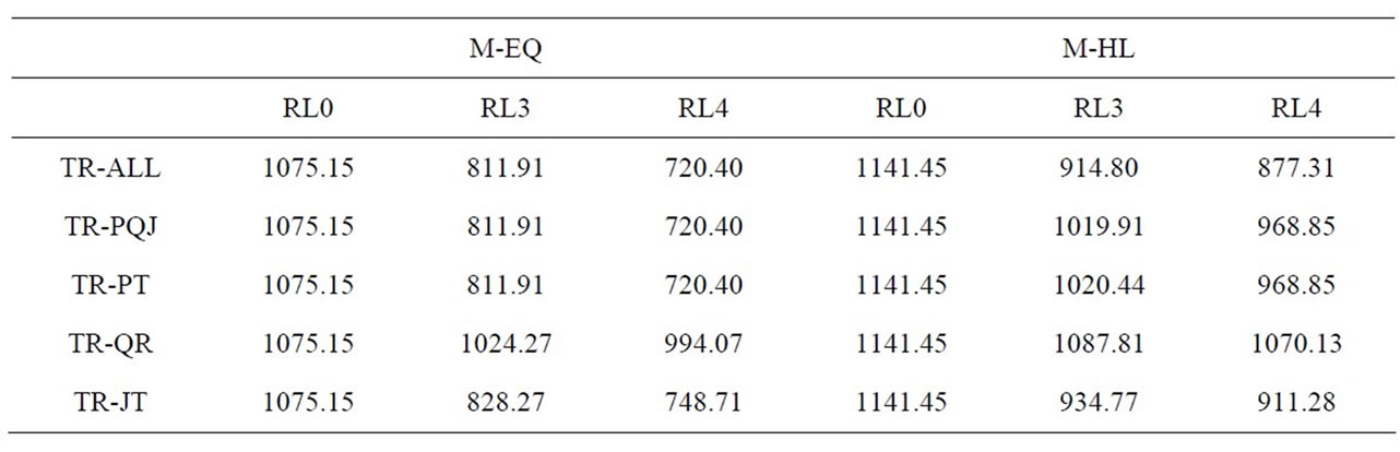
Table 3. Mean Flow Time (FLOW) Results.
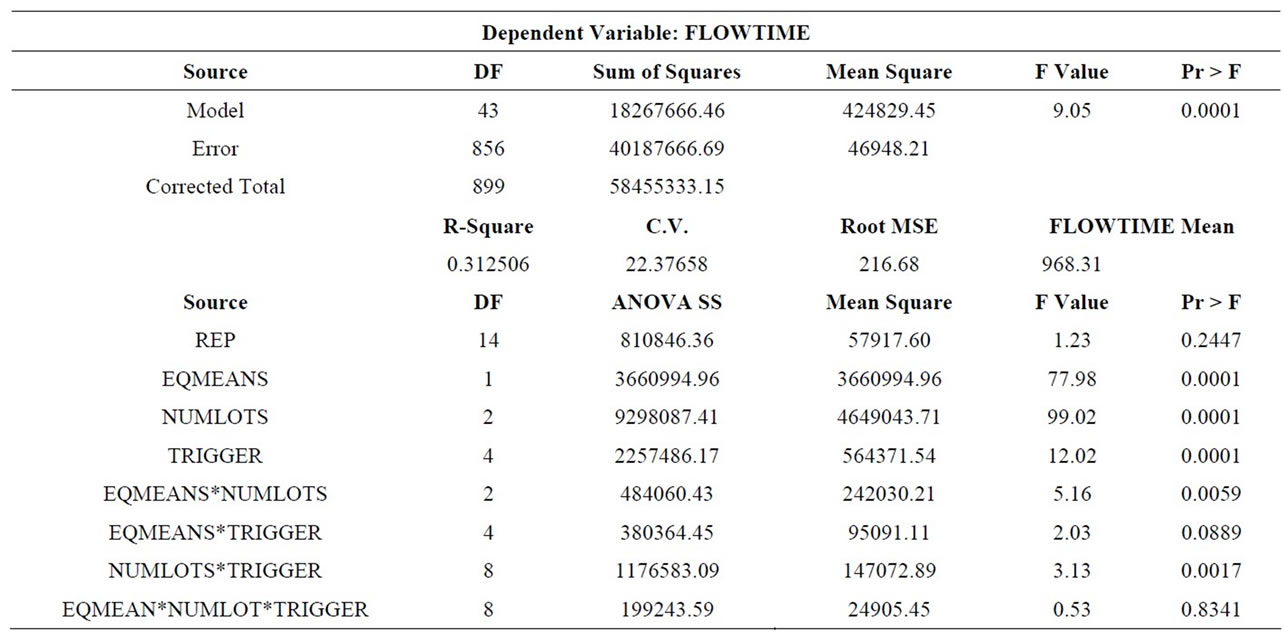
Table 4. Mean Flow Time (FLOW) ANOVA.
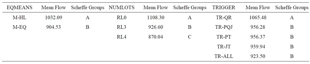
Table 5. Main effects and Scheffe groupings (FLOW).
splitting lots into three and then four sublots substantially improved (reduced) flow time. However, the performance of TR-QR didn’t improve much. The three-way interaction was not significant.
6.2. Standard Deviation of Flow Time (SDFLOW)
The mean standard deviation of flow time for each treatment is given in Table 6, the ANOVA results in Table 7, and the main effects and Scheffe groupings in Table 8. Again, all three main effects were significant and parallel the results for mean flow time. SDFLOW increased approximately 20% when processing means were unequal (M-HL). Conversely, SDFLOW decreased by approximately 10% with the use of lot splitting (either three or four sublots). TR-QR produced a significantly higher SDFLOW than TR-ALL, TR-PT, or TR-PQJ. (TR-JT was not significantly different from any of the others.)
The only interaction which was even marginally significant (p = 0.0967) was NUMLOTS*TRIGGER. The nature of this interaction was the same as for the mean flow time measure: TR-QR was not helped as much by an increased number of sublots as were the other trigger rules.
6.3. Number of Setups (NUMSETS)
Table 9 shows the results for the number of setups per job, the associated ANOVA is shown in Table 10, and Table 11 shows the main effect means and Scheffe groupings. Again, all three main effects were significant. As expected, the number of setups increased significantly when processing means varied across stations (M-HL). Somewhat more interesting was the performance across the number of sublots. Although all levels of this factor were significantly different from each other, the magnitude of the difference between four sublots (4.58 setups per job) and three (4.26 setups per job) is greater than the difference between three sublots (4.26) and no lot splitting (4.13 setups per job). With respect to trigger rules, TR-ALL and TR-JT were significantly worse than the other three.
Each interaction term was also significant. EQMEANS *NUMLOTS was significant because while the number of setups increased when processing means varied across stations and lot splitting was used (RL3 or RL4), it stayed nearly the same (slightly decreased) when lots were not split. The EQMEANS*TRIGGER interaction was significant because when process time means varied
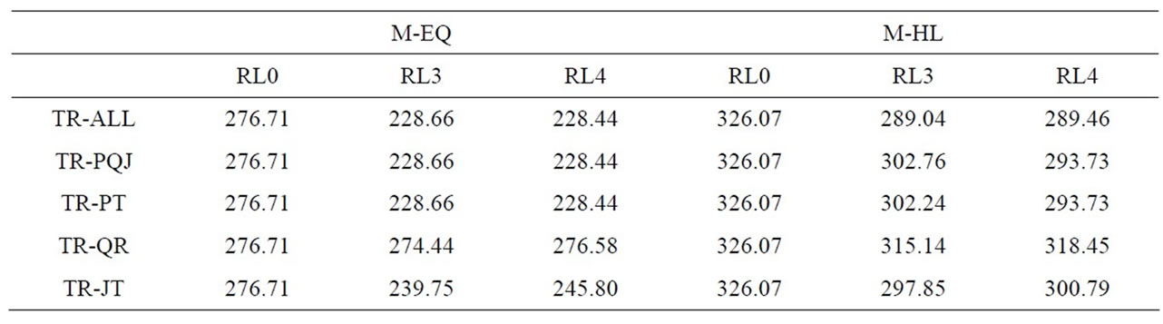
Table 6. Standard deviation of flow time (SDFLOW) results.
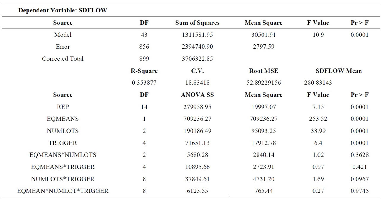
Table 7. Standard deviation of flow time (SDFLOW) ANOVA.
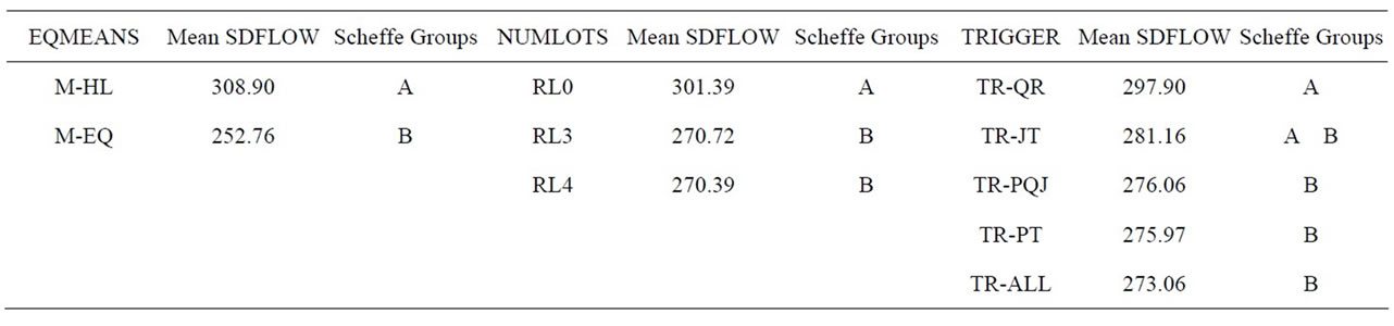
Table 8. Main effects and Scheffe groupings.
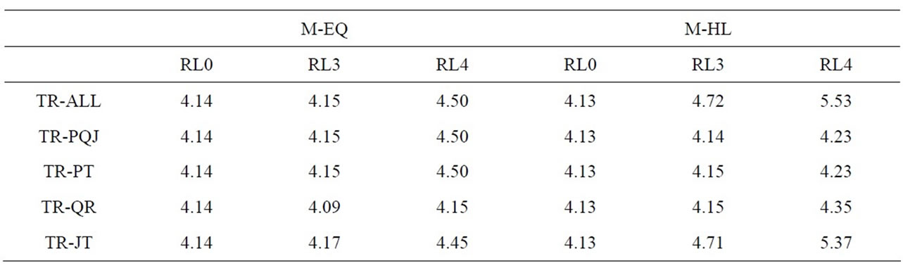
Table 9. Number of setups per job (NUMSETS) results.
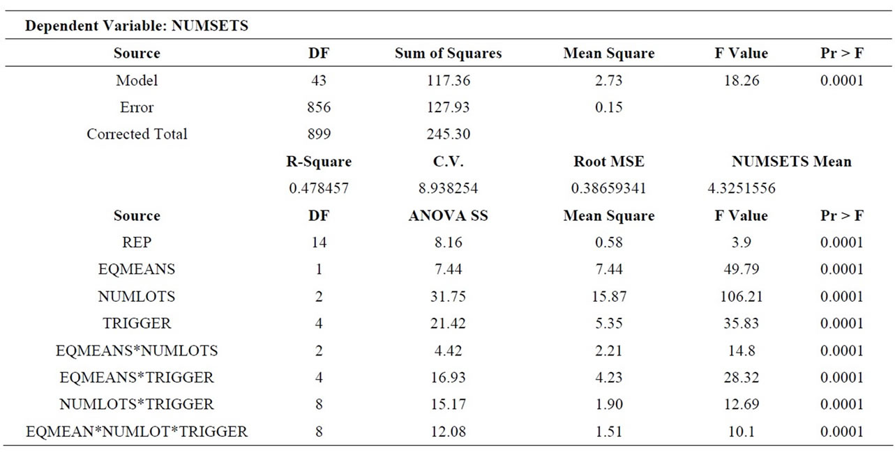
Table 10. Number of setups per job (NUMSETS) results.
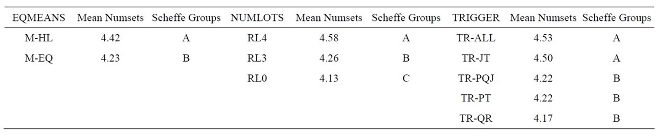
Table 11. Main effects and Scheffe groupings (NUMSETS).
(M-HL), TR-ALL and TR-JT got much worse, TR-QR got only slightly worse, and TR-PT and TR-PQJ got slightly better. This makes sense because the logic of TR-PT (and therefore TR-PQJ) keys on the presence of unequal means. A more important result was the significance of the NUMLOTS*TRIGGER interaction, which is graphically depicted in Figure 4. With TR-ALL and TR-JT, the increase in setups was substantial as lot splitting was used and the number of sublots increased from three to four. The increase for TR-PT, TR-QR, and TR-PQJ was negligible when jobs were first split into three sublots. (The lines for TR-PT and TR-PQJ are superimposed in Figure 4.) Only slightly higher for four sublots, much of this increase may even have been attributable to the small size of the flag sublot.
The three-way interaction term (EQMEANS*NUMLOTS*TRIGGER) was also significant. The reason appears to have been that while M-HL hurt (increased setups) or didn’t change most combinations, it actually helped the TR-PT × RL4 (and TR-PQJ × RL4) combination. This presumably occurred because the small size (one unit) of the flag lot used by RL4 made its ability to “hold a place” for the remainder of the job tenuous. Since so little time was required to process this flag lot, there
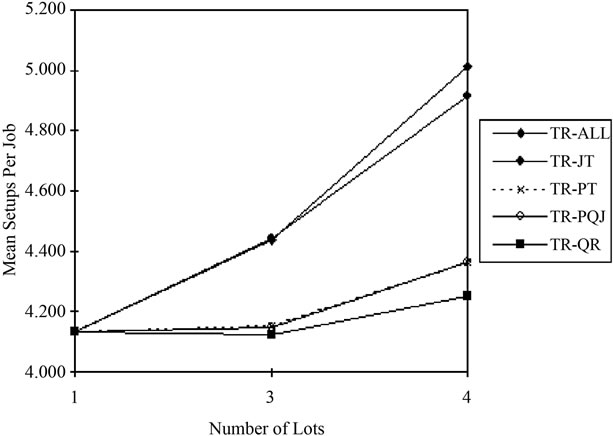
Figure 4. Interaction of lot splitting and trigger rules for NUMSETS.
was plenty of opportunity for it to be finished and get separated from the remainder of its parent job by intervening lots of other job types. In other words, the small size of the flag lot makes it more vulnerable to the type of situation TR-PT was designed to overcome. This result seems to further accentuate the effectiveness of conditional logic.
7. Conclusions and Recommendations
Not surprisingly, our results confirm those of previous research in showing the dramatic improvements in flow time made possible by the use of lot splitting. However, they also demonstrate how lot splitting may lead to significant increases in the number of setups.
The scenario we tested also shows that when the mean processing time varies from station to station, which will often be the case in practice, the potential exists for a significant increase in flow times, negating much of the benefit of lot splitting. Even worse, this same characteristic amplifies the increase in the number of setups incurred by lot splitting schemes. When lot splitting is used in such a scenario, a doubly negative combination exists since both factors contribute to increased setups with much of the flow time advantage of lot splitting lost. The increase in setups is made even more significant by the fact that it was observed when repetitive lots logic was being used, which is specifically intended to avoid setups.
The key role that processing time differentials play in the generation of extra setups has an important general implication for lot splitting schemes which split jobs into unequally sized sublots. As shown by our results for RL4, rules which cause smaller sublots to proceed in advance of larger ones run a greater risk of becoming separated.
However, we have also shown that the use of conditional lot splitting logic may prove effective at retaining most of the flow time advantage of lot splitting and/or avoiding most of the additional setups. With traditional lot splitting, we don’t really know what’s going to happen to a particular job at a particular stage. Instead, we take a risk (split the lot), hope good things will happen (operations will overlap), and take partial precautions (e.g. sequencing by repetitive lots) to guard against the bad things that we know could also happen. Conditional lot splitting is a more thoughtful approach because it starts with the questions of when and why good/bad things happen and tries to use lot splitting everywhere except where the circumstances are most conducive to the generation of additional setups. In this regard, our paper extends the results of Ruben and Mahmoodi [16] to show that selective or conditional splitting of lots can be applied beneficially even when there are multiple imbalances in processing means rather than a single bottleneck.
In summary, we conclude that:
• Lot splitting is not always as advantageous as might be inferred from the results of previous research. Specifically, we have demonstrated realistic circumstances under which flow time improvements diminish.
• By keeping lots split at all operations, lot splitting rules previously considered may incur substantial increases in the number of setups accomplished, even when repetitive lots sequencing is used.
• The use of conditional lot splitting rules (release trigger rules) can achieve a large portion of the flow time improvements of lot splitting, while avoiding most of the additional setups incurred by the unconditional lot splitting schemes previously studied.
7.1. Recommendations for Applying Lot Splitting Rules
Our results show that the TR-PT rule was able to the best job of simultaneously reducing flow times and avoiding additional setups. (Although its more inclusive version, TR-PQJ, performed comparably, its additional complexity was not offset by performance improvements.) As shown graphically in Figure 5 (for the case of unequal processing time means), the performance of the different approaches suggest the possible existence of an “efficient frontier” when flow time and number of setups are considered simultaneously. While not best on either criterion, the RL4 × TR-PT combination was able to achieve over 65% of the flow time reduction of standard lot splitting logic (TR-ALL), while avoiding over 92% of the additional setups incurred by that same logic. For circumstances where process means are not equal and setup costs are a concern, managers should consider applying the TR-PT version of lot splitting.
Although we asserted earlier that we consider conditional logic to be practical, it is fair to ask how it would or could be implemented. Table 12 shows our recommendations. The table indicates that the best method would probably be a function of the shop’s flow pattern and product diversity.
In the simplest case (flow shops with a low variety of products), a manual system or verbal instructions would probably suffice. Since so few cases exist, each station could simply be instructed which product types it is to release in smaller transfer lots and which it should release to the next station as whole jobs.
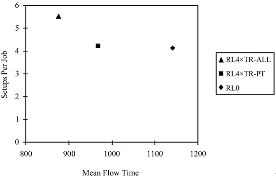
Figure 5. Tradeoff between setups and flow times.
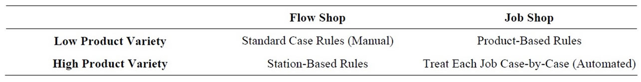
Table 12. Implementation of conditional logic.
Conversely, in the most complex case (job shops with high product variety), it would be necessary to treat each job on a case-by-case basis. However, we believe it is reasonable to expect that systems with this much complexity already rely on automated systems. In such systems, each job’s records could be individually updated in the planning phase to communicate the appropriate decision for each operation, either on-line or on printed routing sheets.
The two intermediate cases (low variety job shops and high variety flow shops) could perhaps establish rules which generalize based on the least diverse dimension. It should be remembered if there are portions of the system where the complexity may be too great, management may simply default to either always or never splitting lots. The benefits of the conditional logic could still be realized in the remainder of the system.
7.2. Recommendations for Future Research
Given the potential benefits of lot splitting, there remains a need for numerous subsequent studies. Important directions include:
• Isolation of other factors contributing to additional setups when lot splitting is used and proposal/testing of appropriate modifications to lot splitting logic.
• Discovery of the extent to which lot splitting policy performance is sensitive to environmental characteristics other than those tested here.
• Consideration of dynamic lot forming rules. While trigger rules permit the timing of lot splits to vary, it is conceivable that benefits might be achieved by permitting the size of split lots to vary throughout the process flow.
• Consideration of policies which require a constant lot size (and vary the number of splits), perhaps due to physical resource constraints such as machine or container capacity.
REFERENCES
- E. M. Goldratt and R. E. Fox, “The Race,” North River Press, Croton-on-Hudson, 1986.
- T. L. Smunt, A. H. Buss and D. H. Kropp, “Lot Splitting in Stochastic Flow Shop and Job Shop Environments,” Decision Sciences, Vol. 27, No. 2, 1996, pp. 215-238.
- doi: 10.1111/j.1540-5915.1996.tb00851.x
- U. S. Karmarkar, S. Kekre and S. Kekre, “Lotsizing in Multi-Item Multi-Machine Job Shops,” IIE Transactions, Vol. 17, No. 3, 1985, pp. 290-297.
- doi:10.1080/07408178508975305
- F. Defersha and M. Chen, “A Hybrid Genetic Algorithm For Flowshop Lot Streaming with Setups and Variable Sublots,” International Journal of Production Research, Vol.48, No. 6, 2010, pp. 1705-1726. doi:10.1080/00207540802660544
- F. Chan, T. Wong and L. Chan, “The Application of Genetic Algorithms to Lot Streaming in a Job-Shop Scheduling Problem,” International Journal of Production Research, Vol. 47, No. 12, 2009, pp. 3387-3412. doi:10.1080/00207540701577369
- D. Biskup and M. Feldmann, “Lot Streaming with Variable Sublots: An Integer Programming Function,” Journal of the Operational Research Society, Vol. 57, No. 3, 2006, pp. 296-303. doi:10.1057/palgrave.jors.2602016
- G. Dobson, U. S. Karmarkar and J. L. Rummel, “Batching to Minimize Flow Times on Parallel Machines,” Management Science, Vol. 35, No. 5, 1989, pp. 607-613. doi:10.1287/mnsc.33.6.784
- S. Dauzere-Peres and J. Lasserre, “Lot Streaming in Job-Shop Scheduling,” Operations Research, Vol. 45, No. 4, 1997, pp. 584-595. doi:10.1287/opre.45.4.584
- D. H. Kropp and T. L. Smunt, “Optimal and Heuristic Models for Lot Splitting in a Flow Shop,” Decision Sciences, Vol. 21, No. 4, 1990, pp. 691-709.
- C. Low, C. Hsu and K. Huang, “Benefits of Lot Splitting in Job-Shop Scheduling,” The International Journal of Advanced Manufacturing Technology, Vol. 24, 2004, pp. 773-780. doi:10.1007/s00170-003-1785-9
- B. Wagner and G. Ragatz, “The Impact of Lot Splitting on Due Date Performance,” Journal of Operations Management, Vol. 12, No. 1, 1994, pp. 13-26. doi:10.1016/0272-6963(94)90003-5
- T. M. Hancock, “Effects of Lot Splitting Under Various Routing Strategies,” International Journal of Operations and Production Management, Vol. 11, No. 1, 1991, pp. 68-74. doi:10.1108/01443579110144277
- C. Liu, “Lot Streaming for Customer Order Scheduling Problem in Job Shop Environments,” International Journal of Computer Integrated Manufacturing, Vol. 22, No. 9, 2009, pp. 890-907. doi:10.1080/09511920902866104
- C. Martin, “A Hybrid Genetic Algorithm/Mathematical Programming Approach to Multi-Family Flowshop Scheduling Problem with Lot Streaming,” Omega: The International Journal of Management Science, Vol. 37, No. 1, 2009, pp. 126-137. doi:10.1016/j.omega.2006.11.002
- J. Buchkin and M. Masin, “Multi-Objective Lot Splitting for a Single Product M-Machine Flowshop Line,” IIE Transactions, Vol. 36, No. 2, 2004, pp. 191-202. doi:10.1080/07408170490245487
- R. A. Ruben and F. Mahmoodi, “Lot Splitting in Unbalanced Production Systems,” Decision Sciences, Vol. 29, No. 4, 1997, pp. 921-949.
- S. M. Shafer and J. M. Charnes, “Cellular versus Functional Layouts under a Variety of Shop Operating Conditions,” Decision Sciences, Vol. 24, No. 3, 1993, pp. 665- 681. doi:/10.1111/j.1540-5915.1993.tb01297.x
- F. Sassani, “A Simulation Study on Performance Improvement of Group Technology Cells,” International Journal of Production Research, Vol. 28, No. 2, 1990, pp. 293-300. doi:10.1080/00207549008942711
- N. C. Suresh, “Partitioning Work Centers for Group Technology: Analytical Extension and Shop-Level Simulation Investigation,” Decision Sciences, Vol. 23, No. 2, 1992, pp. 267-290. doi:10.1111/j.1540-5915.1992.tb00389.x
- S. M. Shafer and J. R. Meredith, “An Empirically Based Simulation Study of Functional versus Cellular Layouts with Operations Overlapping,” International Journal of Operations and Production Management, Vol. 13, No. 2, 1993, pp. 47-62. doi:10.1108/01443579310025303
- V. R. Kannan and S. B. Lyman, “Impact of Family-Based Scheduling on Transfer Batches in a Job Shop Manufacturing Cell,” International Journal of Production Research, Vol. 32, No. 12, 1994, pp. 2777-2794. doi:10.1080/00207549408957099
- F. R. Jacobs and D. J. Bragg, “Repetitive Lots: FlowTime Reductions through Sequencing and Dynamic Batch Sizing,” Decision Sciences, Vol. 19, No. 2, 1988, pp. 281- 294. doi:10.1111/j.1540-5915.1988.tb00267.x
- R. Narasimhan and S. A. Melnyk, “Setup-Time Reduction and Capacity Management: A Marginal Cost Approach,” Production and Inventory Management Journal, Vol. 31, No. 4, 1990, pp. 55-59.
- E. J. Hay, “Any Machine Setup Time Can Be Reduced By 75%,” Industrial Engineering, Vol. 19, No. 8, 1987, pp. 62-67.
- W. J. Hopp and M. L. Spearman, “Factory Physics: Foundations of Manufacturing Management,” Irwin, Chicago, 1996.
- P. D. Welch, “The Statistical Analysis of Simulation Results,” In: S. S. Lavenburg, Ed., Computer Performance Modeling Handbook, Academic Press, New York, 1983.
- A. Z. Szendrovits, “Manufacturing Cycle Time Determination for a Multi-Stage Economic Production Quantity Model,” Management Science, Vol. 22, No. 3, 1975, pp. 298-308. doi:10.1287/mnsc.22.3.298
- G. Dobson, U. S. Karmarkar and J. L. Rummel, “Single Machine Sequencing with Lot Sizing,” Working Paper Series No. QM8419, University of Rochester, Rochester, 1985.
- G. Dobson, U. S. Karmarkar and J. L. Rummel, “Batching to Minimize Flow Times on One Machine,” Management Science, Vol. 33, No. 6, 1987, pp. 784-799. doi:10.1287/mnsc.33.6.784
- U.S. Karmarkar, S. Kekre, S. Kekre and S. Freeman, “Lot-Sizing and Lead-Time Performance in a Manufacturing Cell,” Interfaces, Vol. 15, No. 2, 1985, pp. 1-9. doi:10.1287/inte.15.2.1
- C. Santos and M. J. Magazine, “Batching in Single Operation Manufacturing Systems,” Operations Research Letters, Vol. 4, No. 3, 1985, pp. 99-102. doi:10.1016/0167-6377(85)90011-2
- J. P. Moily, “Optimal and Heuristic Procedures for Component Lot-Splitting In Multi-Stage Manufacturing Systems,” Management Science, Vol. 32, No. 1, 1986, pp. 113-125. doi:10.1287/mnsc.32.1.113
- S. C. Graves and M. M. Kostreva, “Overlapping Operations in Material Requirements Planning,” Journal of Operations Management, Vol. 3, No. 2, 1986, pp. 283-294. doi:10.1016/0272-6963(86)90004-5
- D. Trietsch and K. Baker, “Basic Techniques for Lot Streaming,” Operations Research, Vol. 41, No. 6, 1993, pp. 1065-1076. doi:10.1287/opre.41.6.1065
- K. Baker, “Lot Streaming in the Two-Machine Flow Shop with Setup Times,” Annals of Operations Research, Vol. 57, No. 1, 1995, pp. 1-11. doi:10.1007/BF02099687