Modern Instrumentation
Vol.1 No.3(2012), Article ID:21063,7 pages DOI:10.4236/mi.2012.13004
Pass/Fail Criterion for a Simple Radiation Portal Monitor Test
1Statistical Sciences, Los Alamos National Laboratory, Los Alamos, USA
2Neutron Science Center, Los Alamos National Laboratory, Los Alamos, USA
Email: tburr@lanl.gov
Received April 28, 2012; revised June 1, 2012; accepted June 20, 2012
Keywords: Poisson Distribution; Radiation Portal Monitor; Tolerance Interval
ABSTRACT
One of the simplest tests of a radiation portal monitor (RPM) is a series of n repeats (a vehicle drive-through) in which the ith repeat records a total number of counts Xi and alarms if Xi ≥ T where T is an alarm threshold. The RPM performance tests we consider use n repeats to estimate the probability p = P(Xi ≥ T). This paper addresses criterion A for testing RPMs, where criterion A is: for specified source strength, we must be at least 95% confident that p ≥ 0.5. To assess criterion A, we consider a distribution-free test and a test relying on assuming the counts Xi have approximately a Poisson distribution. Both test options require tolerance interval construction.
1. Introduction
This paper considers testing the response of a specific radiation portal monitor (RPM) to a specified source being transported in a vehicle. One of the simplest tests of an RPM is a series of n repeats (a vehicle drive-through) in which the ith repeat records a total number of counts Xi and alarms if Xi ≥ T, where T is an alarm threshold. The RPM performance tests we consider use n repeats to estimate the probability p = P(Xi ≥ T). This paper addresses criterion A for testing RPMs, where criterion A is: for specified source strength, we must be at least 95% confident that p ≥ 0.5. To assess criterion A, we consider a distribution-free test and a test relying on assuming the counts Xi have approximately a Poisson distribution. Both test options require tolerance interval construction. The following sections include additional background, statistical models and assumptions, numerical examples, and extensions.
2. Background
Radiation detection systems are deployed at ports of entry into the U.S. to protect against entry of illicit nuclear and radiological materials or so-called threat sources [1]. Radiation Portal Monitors (RPMs) are passive, non-intrusive devices used to screen vehicles, containers, and other conveyances for Special Nuclear Materials (SNM) such as uranium and plutonium. These materials emit neutrons and/or gamma rays (or gammas), which many RPMs aim to detect using Helium-3 (3He) tubes for neutrons and plastic scintillator and other materials for gammas. A gamma detector not only counts gammas but also measures their associated energies. In some deployments, the gamma counts are coarsely binned into low and high energy channels. In others using plastic scintillator detector material, the gamma counts are less coarsely binned into approximately eight energy channels [2].
Data from these passive RPMs have been collected at various ports of entry since 2003 [2-6]. As a vehicle slowly passes by a set of fixed radiation sensors, a time series of measurements from each sensor is recorded. The most common sensor configuration for vehicular RPMs consists of top and bottom panels on both the driver’s side and passenger’s side, with each panel containing a neutron counter and a gamma counter that records every 0.1 second during a “vehicle profile”; a vehicle screening lasts approximately 10 to 30 seconds depending on the vehicle speed, resulting in approximately 100 to 300 data records per vehicle profile.
An important issue in fielding RPMs is that an RPM vendor must be selected among viable candidates. One of the simplest tests of an RPM is a series of n repeats (a vehicle drive-through) in which the ith repeat records a total number of counts Xi and alarms if Xi ≥ T, where T is an alarm threshold. The RPM performance tests we consider use n repeats to estimate the probability p = P(Xi ≥ T). This paper addresses criterion A for testing RPMs, where criterion A is: for a specified source strength, we must be at least 95% confident that p ≥ 0.5. To assess criterion A, we consider a distribution-free test and a test relying on assuming the counts Xi have approximately a Poisson distribution. Our experience suggests there is some misunderstanding regarding tolerance interval construction, which is required in either test for criterion A.
2.1. RPM Testing Criteria
We begin with definitions of RPM testing criteria as used in several vendor selection experiments.
Definitions: Drive-through: In a drive-through, a vehicle drives by a portal at a required speed. We refer to a drive-through as a “repeat”.
Portal monitor test: A portal monitor test consists of series of n repeats. The portal registers a number of counts, Xi, for repeat i (i = 1, ··· n). In the following, we will consider n = 20, but the results can be generalized for any n.
Alarm: Each time a repeat results in Xi ≥ T where T is an alarm threshold, we call it an “alarm” and define the alarm probability p = P(Xi ≥ T).
For selection of portal monitors we consider criterion A, defined as: Criterion A: be at least 95% confident that p ≥ 0.5. We consider two possible tests of criterion A.
2.2. Tolerance Intervals
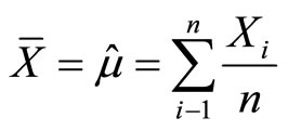
Researchers in the physical sciences are usually familiar with the concept of a confidence interval (CI). For example, the sample mean ![]() and the sample standard deviation s of a sample of size n can together be used to construct an approximate 95% CI for the true population mean using
and the sample standard deviation s of a sample of size n can together be used to construct an approximate 95% CI for the true population mean using
where
is the  percentile of the t distribution with n – 1 degrees of freedom.
Somewhat similarly to a confidence interval, a tolerance interval is an interval within which, with some confidence level, a specified proportion of a population falls. If a population’s parameters were known exactly, one could compute a range within which a certain proportion of the population falls. For example, if we know that a population is normally distributed with mean μ and standard deviation σ, then the interval μ ± 1.96σ includes 95% of the population. However, in most situations, we know only the sample mean  and sample standard deviation
 , which are only estimates of the true parameters. In that case,
  will not necessarily include 95% of the population, because of variability (across hypothetical replicates of obtaining n observations) in
  and
and . A tolerance interval bounds this variability by introducing a confidence level γ, which is the confidence with which this interval actually includes the specified proportion of the population. Calculations and software for computing approximate tolerance intervals for various distributions are available for example by Young [7].
In this paper, we first assume the RPM counts have a Gaussian distribution. Note that counts are integer-valued so a better model (see Appendix 1) is the familiar Poisson distribution. However, provided the mean μ of the Poisson is large, say 30 or higher, the Gaussian is an adequate approximate to the Poisson. For completeness, Section 2.5 considers the case of RPM counts having a Poisson distribution.
2.3. Test Options for Criterion A
2.3.1. Test Option “1” for Criterion A: A Nonparametric “Sign” Test
Using standard binomial sampling theory and the Clopper-Pearson so-called “exact” method of confidence interval construction [7], we find that if

for n = 20 then criterion A is satisfied, where the indicator I (Xi ≥ T) = 1 if Xi ≥ T and 0 otherwise. In other words, this test option to meet criterion A simply requires 15 or more alarms in n = 20 repeats.
As an aside, if instead of a 95% confidence interval for p we tested the hypothesis H0: p ≥ 0.5, this test option would change to require only 14 or more alarms in n = 20 repeats. To be conservative, we use the 15 or more alarms requirement as test option 1.
2.3.2. Test Option “2” for Criterion A: A Parametric Mean and Standard Deviation Test
We assume here that Xi has a normal (Gaussian) distribution with mean μ and variance σ2, which is a good assumption provided the mean count rate is large so the Gaussian provides a good approximation to the Poisson distribution.
Record the number of counts Xi in each repeat and calculate the sample average
and the sample variance

where the “hat” notation denotes that the quantity is an estimate of a population parameter, in this case, the population mean μ and variance σ2. Standard tolerance interval construction can be used to show that 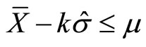 with probability 0.95 for k = 0.3866. This test option is therefore
 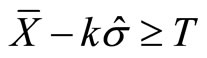 because the symmetry of the Gaussian distribution implies that if μ = T, then p ≥ 0.5.
NOTE 1: We have verified the Clopper-Pearson result for test option 1 using the binconf function in R [8] and verified the tolerance interval result k = 0.3866 using simulation in R.
NOTE 2: A summary of test options 1 and 2 is as follows.
Test option 1 is a “nonparametric” test and it requires at least 15 passes in 20 trials.
Test option 2 is a “parametric” test and it requires .
.
Using either option 1 or 2, if the criterion is met, then with probability at least 0.95, p ≥ 0.5.
2.4. Requirement for a 95% Pass Rate
Suppose for cost reasons it is desirable to have a high pass rate for RPMs. Then it is useful to evaluate the size of compared to the alarm threshold T so that test option 1 (or option 2) results in a “pass” with high probability (we will use 0.95).
2.4.1. Test Option “1” for Criterion A: Requirement for a 95% Pass Rate
In order for
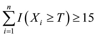
with probability 0.95, standard binomial calculations (we used pbinom in R) imply that p ≥ 0.86.
Next, in order for p = P(Xi ≥ T) ≥ 0.86, we require μ ≥ T + 1.0803σ. Recall that we assume Xi ~ N(μ, σ2), so the factor 1.0803 is the 0.86 quantile of the normal distribution, which we calculated using qnorm in R.
Therefore, provided Xi ~ N(μ, σ2) and μ ≥ T + 1.0803σ, criterion A will be met (by having at least 15 alarms in n = 20 repeats) with probability at least 0.95.
2.4.2. Test Option “2” for Criterion A: Requirement for a 95% Pass Rate
Recall that tolerance interval construction for the Gaussian distribution can be used to show that  with probability 0.95 for k = 0.3866. If we require
  for test option 2, then by the same tolerance interval calculation (which we again verified by simulation in R), if μ ≥ T + 2 × 0.3866 × σ then criterion A is met with probability at least 0.95.
In summary, the requirement for μ is μ ≥ T + 1.083 × σ for the nonparametric test and μ ≥ T + 0.77 × σ for the parametric test. Therefore, the lower limit of detection is smaller for the parametric test, which is not surprising because it makes more assumptions about the underlying distribution.
2.5. Criteria for Options 1 and 2 for Poisson Data
The key issue with Poisson data is that the Poisson variance depends on mean; specifically, if X ~ Pois(μ) then σ2 = μ. By symmetry of the Gaussian, we need μ ≥ T in order for p ≥ 0.5. For any underlying distribution, we need p = P(X ≥ T) ≥ 0.86. It is simple to verify numerically (see Figure 1) that provided μ ≥ 1, then P(X ≥ μ) ≥ 0.5. Therefore, as with the Gaussian case, we will convert assessment of whether P(X ≥ μ) ≥ 0.5 to assessment of whether μ ≥ T which results in a conservative approach, requiring a slightly larger mean count rate µ than is actually necessary to meet the criterion.
2.5.1. Test Option “1” for Criterion A: A Nonparametric “Sign” Test
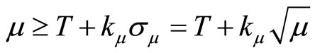
As with the Gaussian assumption, we require 15 or more alarms, which occurs with probability 0.95 or higher if p = P(X ≥ T) ≥ 0.86 as test option 1. In order for p ≥ 0.86, recall that we need μ ≥ T + 1.0803σ for the Gaussian case. For the Poisson case, we require
 .
.
We have found by simulation in R (see Appendix 2) that kμ ≤ 1.0803, and that it is too conservative to simply use the 1.0803 value that is appropriate for the Gaussian case. For example, if μbkg =2, 10, or 40 (2 to 40 is approximately the range of the count rate per second across world-wide RPM deployments of the same type of neutron detector) and
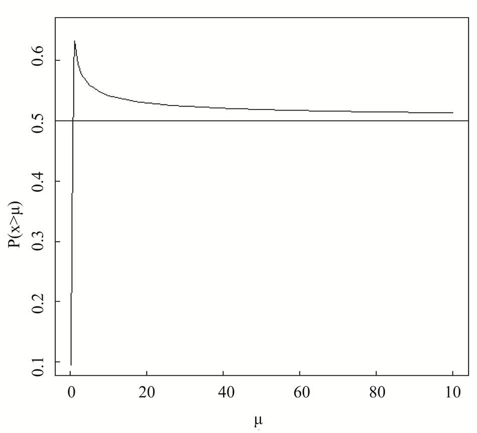
Figure 1. The probability that X > μ for a range of μ values.

(see Section 4), then
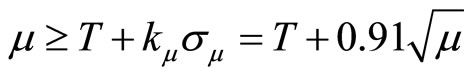 .
.
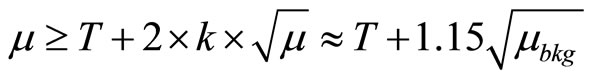
Recall that in the Gaussian case, provided Xi ~ N(μ, σ2) and μ ≥ T + 1.0803σ, criterion A will be met (by having at least 15 alarms in n = 20 repeats) with probability at least 0.95. In the Poisson case if we re-express the requirement for μ in terms of the background mean rather than the background + signal mean, then μ ≥ T + kμμbkg then kμ is approximately 1.38 rather than 0.91 for μbkg =10. The mean reasons that the Poisson model has a different kμ than k for the Gaussian are: 1) the variance of the Poisson distribution can be estimated with lower error (by using the sample mean rather than the sample variance) than can the variance of the Gaussian, and 2) the Poisson variance equals the poisson mean.
2.5.2. Test Option “2” for Criterion A: A Parametric Mean and Standard Deviation Test
If X has a Poisson distribution with mean µ then an optimization method in R (see Appendix 2) shows that for μ = 2, 10, and 40, we require k = 0.36, 0.36, and 0.35, respectively, in the expression
for μbkg = 10. Recall that the value of k for the Gaussian distribution is k = 0.3866. Because the k values for the Poisson for μ ranging from 2 to 40 are all very close and slightly less than the required value of k for the Gaussian, it is adequate to simply use the value k = 0.3866 that is also used for the Gaussian. The reason the k values for the parametric Poisson case are so close that the k value for the Gaussian case is that the values of m are reasonably large (larger than 1 for example) and the central limit theorem suggests that the average of n = 20 Poisson repeats will therefore have approximately a Gaussian distribution.
In summary, the requirement for the case is
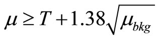
for the nonparametric test and
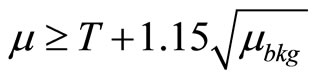
for the parametric test.
Therefore, again the lower limit of detection is smaller for the parametric test, which is not surprising because it makes more assumptions about the underlying distribution.
3. Estimation of the Threshold T
We have assumed the threshold T is known without error and that it corresponds to some user-specified small false alarm probability (FAP). For example, Figure 2 plots the value of T needed for a 0.001 FAP for a range of background averaging times for μ = 2, 8, and 40 counts per second (approximately the range observed in similar RPMs deployed worldwide). These values were obtained by simulation in R [8].
It is impractical to allow 100 seconds for a background measurement prior to each repeat. Fortunately, the true mean μ drifts slowly with time [5,6]. For example, Figure 3 shows a smooth curve through the estimated value μ prior to each profile in real data. Because the mean μ is slowly varying, a running average is used to estimate the current μ, using some combination of the current estimate and the newest estimate from each profile using approximately 1 second of new background counts prior to each profile. Figure 4 shows the mean squared estimation error in estimating the background μ as a function of the background averaging time using the local mean (obtained just prior to the profile).
The mean squared estimation errors in Figure 4 were estimated by assuming the smooth curve in Figure 3 is the true slowly-varying mean, say μt, generating Poisson observations having mean μt, and using either the local mean estimated just prior to each profile to estimate μt. Figure 5 is similar to Figure 4, but shows that a running mean (using 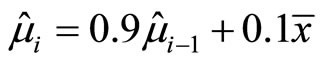 as the running mean, where
 ![]() is the local mean) has smaller estimation error than the local mean.
is the local mean) has smaller estimation error than the local mean.
In practice, T is estimated using an estimate of the background and either Gaussian or Poisson probabilities to estimate the FAP. Estimation error in T can be viewed in our context as leading to estimation error in the FAP, but provided the running mean approach is used, that estimation error in the FAP is quite small.

Figure 2. Alarm threshold k for 0.001 false alarm rate as a function of the duration of the background averaging period for 3 background means (2, 8, and 40 cps).
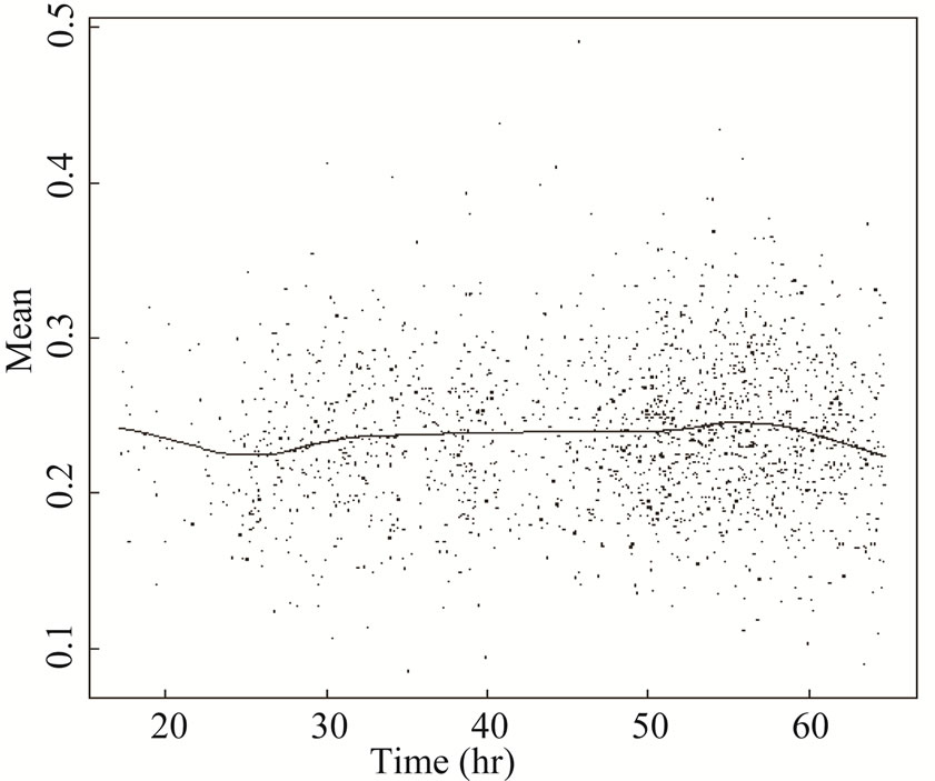
Figure 3. Example of real neutron average counts over approximately 48 hours.
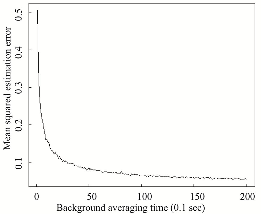
Figure 4. The mean squared estimation error as a function of the background averaging time in 0.1 seconds.
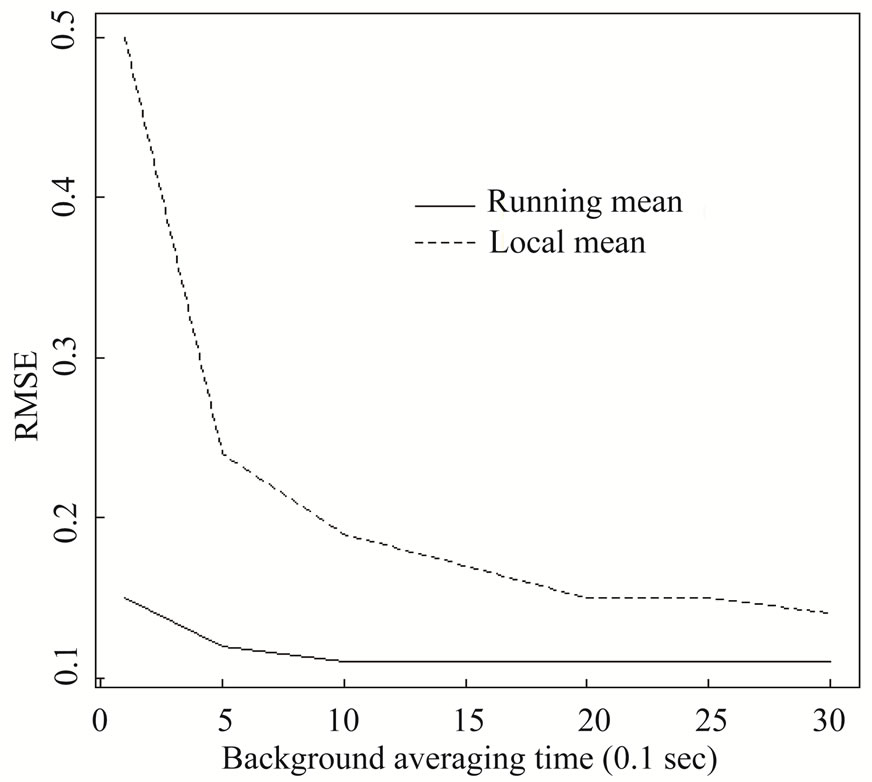
Figure 5. The mean squared estimation error as a function of thebackground averaging time in 0.1 seconds using either a running mean or the local mean for the slowly varying real data shown in Figure 4.
4. Discussion and Summary
An important issue in fielding RPMs is that an RPM vendor must be selected among viable candidates. This paper supports experiments aimed to test RPMs prior to vendor selection. One of the simplest tests of an RPM is the “≥15 alarms in 20 repeats” rule, which arose from criterion A that requires at least 95% confidence that Xi ≥ T, where T is an alarm threshold, with at least 0.50 probability. Note that even if a test has ≥15 alarms in 20 repeats, we cannot claim that with probability 0.95, future Xi ≥ T with at least 0.50 probability. That’s why the term “confidence” is used, and it arises from defensible use of binomial probabilities. In fact, it is possible that the true P(Xi ≥ T) < 0.50 for ALL vehicles that pass the ≥15 alarms in 20 repeats rule (although the pass rate would be low).
We have provided a non-parametric and a parametric option for both the Gaussian and the Poisson models for criterion A. The numerical values required to implement these options are summarized in Sections 2.3 and Sections 2.5 and were estimated using a simple optimization function freely available in R, with example R code given in Appendix 2.
Typically the alarm threshold T is estimated from the background data, so we included an assessment of the actual versus the nominal false alarm probability as a function of the background averaging period.
We also added a practical requirement involving the RPMs detected count rate µ such that that vehicles pass the test with probability at least 0.95. We did not consider the signal shape during the profile, because either the vehicle is assumed stationary, or the total neutron counts over the entire profile are used. References [4,5, 9,10] provide analyses appropriate for alarm rules that do consider signal shape during the profile.
5. Acknowledgements
We acknowledge the Department of Homeland Security for funding the production of this material under DOE Contract Number DE-AC52-06NA25396 for the management and operation of Los Alamos National Laboratory.
REFERENCES
- B. Geelhood, J. Ely, R. Hansen, R. Kouzes, J. Schweppe and R. Warner, “Overview of Portal Monitoring at Border Crossings,” 2003 IEEE Nuclear Science Symposium Conference Record, Portland, 19-25 October 2003, pp. 513- 517. doi:10.1109/NSSMIC.2003.1352095
- J. Ely, R. Kouzes, J. Schweppe, E. Siciliano, D. Strachan and D. Weier, “The Use Of Energy Windowing to Discriminate SNM from NORM in Radiation Portal Monitors,” Nuclear Instruments and Methods in Physics Research A, Vol. 560, No. 2, 2005, pp. 373-387. doi:10.1016/j.nima.2006.01.053
- T. Burr, J. Gattiker, M. Mullen and G. Tompkins, “Statistical Evaluation of the Impact of Background Suppression on the Sensitivity of Passive Radiation Detectors,” Springer, New York, 2006.
- T. Burr, J. Gattiker, K. Myers and G. Tompkins, “Alarm Criteria in Radiation Portal Monitoring,” Applied Radiation and Isotopes, Vol. 65, No. 5, 2007, pp. 569-580. doi:10.1016/j.apradiso.2006.11.010
- T. Burr and M. Hamada, “The Performance of Neutron Alarm Rules in Radiation Portal Monitoring,” in revision for Technometrics, 2012.
- R. Kouzes, E. Siciliano, J. Ely, P. Keller and R. McConn, “Passive Neutron Detection For Interdiction Of Nuclear Material At Borders,” Nuclear Instruments and Methods in Physics Research A, 584, No. 2-3, 2008, pp. 383-400. doi:10.1016/j.nima.2007.10.026
- D. Young, “Tolerance: An R Package for Estimating Tolerance Intervals,” Journal of Statistical Software, Vol. 36, No. 5, 2010. www.jstatsoft.org
- R Development Core Team. R: A Language and Environment for Statistical Computing. R Foundation for Statistical Computing, Vienna, 2004. http://www.R-project.org
- S. Robinson, S. Bender, E. Flumerfelt, C. LoPresti, M. Woodring, “Time Series Evaluation of Radiation Portal Monitor Data for Point Source Detection,” IEEE Transactions on Nuclear Science, Vol. 56, No. 6, 2009, pp. 3688-3693. doi:10.1109/TNS.2009.2034372
- T. Schroettner, P. Kindl and G. Presle, “Enhancing Sensitivity of Portal Monitoring at Varying Transit Speed,” Applied Radiation and Isotopes, Vol. 67, No. 10, 2009, pp. 1878-1886. doi:10.1016/j.apradiso.2009.04.015
Appendix 1. The Distribution of the Detected Counts D.
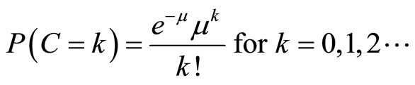
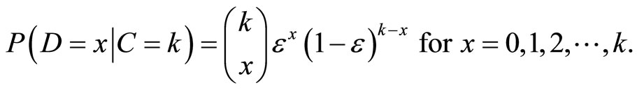
Assume the true counts C have a Poisson distribution with mean µ, so C ~ Poisson(m). Given a realization C, the detected counts D have a binomial distribution with mean , where the detector efficiency e < 1, so
  ~ binomial(C, e). This appendix shows that the unconditional distribution of the detected counts D is Poisson(me).
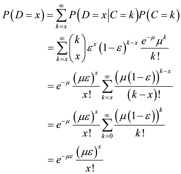

Therefore, 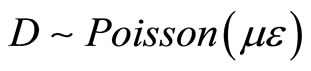
Appendix 2. R Code to Use Simulation in Repeated Calls to the Optimize Function
f2 = function(k = 2, mu = 500, n = 20, sig = 30, lprob = .05, nsim = 1000, do.normal = FALSE){
temp2 = mu
for(isim in 1:nsim) {
x = rpois(n = n, lambda=mu)
# assume Poisson unless # do.normal == TRUE temp1[isim] = mean(x) - k*mean(x)^.5 if(do.normal) {x = rnorm(n = n, mean = mu, sd = sig); temp1[isim] = mean(x) - k*var(x)^.5}
}
abs(1-lprob-mean(temp1 <= temp2))
}
Example result:
optimize(f2, interval = c(0.1,1), nsim = 10^5, mu = 2, n = 20, maximum = FALSE, lprob = 0.05)
$minimum
[1] 0.3648825
Grid search for parametric option
mu.grid = seq(4, 10, length = 10)
k = 0.3866; mu = 2 nsim = 10^5; thresh = 4*mu^.5 + mu grid.save1 = numeric(length(mu.grid))
for(i in 1:length(mu.grid)) {
mutemp = mu.grid[i]
temp2 = thresh
temp1 = numeric(nsim)
for(isim in 1:nsim) {
x = rpois(n=n,lambda=mutemp)
temp1[isim] = mean(x) - k*mean(x)^.5
}
grid.save1[i] = mean(temp1 >= thresh)
}