Open Journal of Statistics
Vol.1 No.1(2011), Article ID:4700,9 pages DOI:10.4236/ojs.2011.11004
Bayes Prediction of Future Observables from Exponentiated Populations with Fixed and Random Sample Size
Department of Mathematics, Alexandria University, Egypt
E-mail: dr_essak@hotmail.com
Received March 22, 2011; revised April 4, 2011; accepted April 14, 2011
Keywords: Predictive Density And Survival Functions, OneAnd Two-Sample Schemes, Bayes Prediction, Exponentiated Population. Exponentiated Burr Type XII Distribution, Data Of Carbon Fibers
Abstract
Bayesian predictive probability density function is obtained when the underlying pop-ulation distribution is exponentiated and subjective prior is used. The corresponding predictive survival function is then obtained and used in constructing 100(1 – t)% predictive interval, using oneand twosample schemes when the size of the future sample is fixed and random. In the random case, the size of the future sample is assumed to follow the truncated Poisson distribution with parameter λ. Special attention is paid to the exponentiated Burr type XII population, from which the data are drawn. Two illustrative examples are given, one of which uses simulated data and the other uses data that represent the breaking strength of 64 single carbon fibers of length 10, found in Lawless [40].
1. Introduction
The general problem of prediction may be described as that of inferring the values of unknown observables (future observations, known as future sample), or functions of such variables, from current available observations, known as informative sample. the problem of prediction can be solved fully within Bayes framework (Geisser [33] ). Bernardo and Smith [22] stated that: “inference about parameters is thus seen to be a limiting form of predictive inference about observables”.
Bayesian prediction bounds for order statistics of future observables from certain distributions, such as the exponential, Rayleigh, Weibull, Pareto and Lomax distributions, have been studied by several authors. See, for example, Dunsmore [27], Lingappaiah [44], Evans and Nigm [28]-[30], Sinha and Howlader [58], Howlader [36], Sinha [56], Raqab [54], Malik [46], Zellner [64], Lwin [43], Sinha and Howlader [57], Arnold and Press [20], Geisser [32], Nigm and Hamdy [50], AL-Hussaini and Jaheen [16], AL-Hussaini [5] and Nigm et al [51]. Prediction bounds for certain order statistics of samples from Burr type XII population, were obtained by Nigm [49], AL-Hussaini and Jaheen [14,15] and Ali Mousa and Jaheen [19]. Prediction bounds, based on heterogeneous populations that can be represented by finite mixtures were developed by Jaheen [37], AL-Hussaini [3], [6] among others.
Prediction was reviewed by Patel [52], Nagaraja [48], Kaminsky and Nelson [38] and AL-Hussaini [4].
Adding one, or more, parameters to a distribution makes it richer and more flexible for modeling data. There are several ways of adding one or more parameters to a distribution. A positive parameter was added to a general survival function (SF) by Marshall and Olkin [47]. In their consideration of a countable mixture of a Pascal(r,p) mixing proportion and positive integer powers of SFs, a SF with two extra parameters was obtained by AL-Hussaini and Ghitany [10]. A new family of distributions as a countable mixture with Poisson added parameter was constructed by AL-Hussaini and Gharib [9]. A simple way of adding a parameter to a distribution is by exponentiation. This goes back to Verhulst [62], who raised his 1838 [61] logistic cumulative distribution function (CDF) to a positive power. Ahuja and Nash [1] seemed to have been the first to raise Verhulst [63] exponential CDF to a positive power.
The exponentiated model is also known as proportional reversed hazard rate model, see Gupta and Gupta [35] or Lehman alternatives, when a is a positive integer, see Lehmann [41].
 (1.1)
(1.1)
where  is a CDF and a is a positive parameter,
  may be a vector and
  where
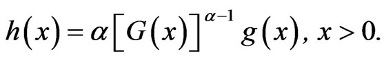
where  is the parameter space. In this paper, we shall assume that G(x) is an absolutely continuous CDF defined on the positive half of the real line. So that, its corresponding probability density function (PDF) is
 . If
. If  is the PDF corresponding to H(x), then
 (1.2)
(1.2)
AL-Hussaini [7] studied some of the properties of the exponentiated distributions where the baseline distribution G is a general CDF. AL-Hussaini [8] estimated the parameters, SF and hazard rate function (HRF) under the general exponentiated model, using maximum likelihood and Bayes methods. He also obtained prediction bounds of future observables based on the two-sample scheme under the exponentiated model.
AL-Hussaini and Hussein [11] estimated the parameters of the exponentiated Burr XII(a, β, g) population when the data are subjected to type II censoring. Maximum likelihood (ML) and Bayes methods were used for estimation. The ML and Bayes estimates were compared when the Bayes estimates are based on square error and linear-exponential loss functions.
In Section 2, the one-sample scheme is used to predict future observables from exponentiated populations. In Section 3, future observables from exponentiated populations are predicted, using two-sample scheme, when the size of the future sample is fixed and when it is random. In Section 4 the results obtained in Sections 2 and 3 are applied to the exponentiated Burr type XII population. In Section 5, Numerical examples are given to illustrate our results.
2. One-Sample Prediction
Suppose that  are the first r ordered life times in a random sample of n components whose failure times are identically distributed as a random variable X having the exponentiated distribution, given by (1.1). Bayesian one-sample prediction is made for some order statistics of the remaining n-r life times. For such remaining n-r components, let
  denote the life time of the sth component to fail, where
 . Write
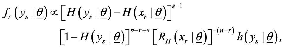
  to denote the conditional PDF of the sth component to fail, given that r components had already failed. Then
The binomial expansion of each of the first three terms on the right hand side then yields
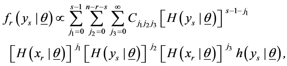
where
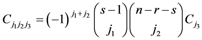 (2.1)
(2.1)
 .(2.2)
Substituting and
and 
 we then have
where
 (2.3)
(2.3)
We shall rewrite  in the form

(2.4)
where
 (2.5)
(2.5)
The predictive PDF of  is defined by
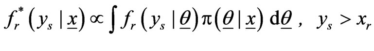 (2.6)
(2.6)
where  is the posterior PDF of
 , given
 . The posterior PDF is such that
 (2.7)
(2.7)
where  is the likelihood function and
  is a prior PDF of
 .
.
Substitution of (2.4) and (2.7) in (2.6), then yields the predictive PDF of the future order statistic
Suppose that the CDF  depends on an unknown k-dimensional vector of parameters
 , so that
  depends on the
(k + 1) unknown parameters . Suppose that
  and
and  are independent so that the prior belief of the experimenter is given by
 (2.8)
(2.8)
where  is gamma
  distribution and
  is a k-variate PDF.
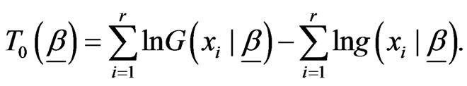
The likelihood function is given by:
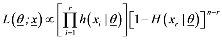
Substitution of (1.1) and (1.2) then yields
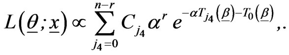
where
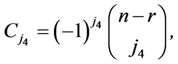
 (2.9)
(2.9)
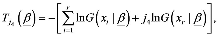
 (2.10)
The posterior PDF of 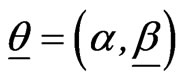 given the data, is then given by
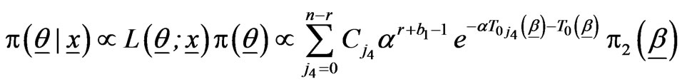
(2.11)
where
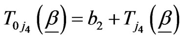 (2.12)
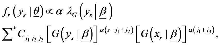
Therefore, the predictive PDF of  is given by
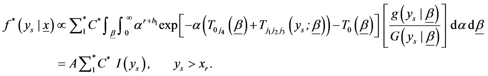
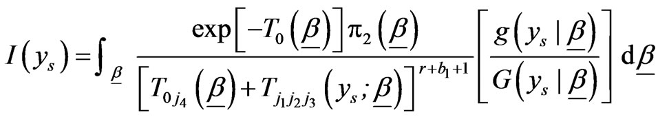
where
 (2.13)
 is given by (2.2), and
It then follows that the predictive SF of  is given by
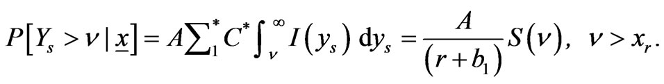
where

 ,
, and
and  are given, respectively, by (2.5) , (2.10) and (2.12).
Notice that:
So that
 (2.14)
A two sided 100(1- ...predictive interval for  is given by
 , where L and U are the solution of the equations
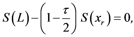 (2.15)
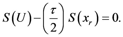 (2.16)
REMARKS
1) A one-sided 100(1- ...predictive interval of the form  is such that L is the solution of (2.15) after replacing
  by
by . Similarly, a one-sided 100(1 – τ)% predictive interval of the form
  is such that U is the solution of (2.16) after replacing
  by
by .
.
2) Equations (2.15) and (2.16) are generally not obtainable analytically and some iteration scheme is used for their solution.
3. Two-Samples Prediction
Suppose that  are the first r ordered life times in a random sample of n components (type II censoring) whose failure times are identically distributed as a random variable X having the exponentiated distribution, given by (1.1). Bayesian prediction is made for
 , the l th ordered lifetime in a future sample of size m (two-sample prediction),
 . The sample size m is assumed to be fixed or random.
4.1. Fixed Sample Size
Suppose that the CDF  depends on an unknown k-dimensional vector of parameters
 , so that
  depends on the
(k + 1) unknown parameters . Suppose that
  and
and  are independent so that the prior belief of the experimenter is given by (2.8). Then the predictive PDF and SF of the future
  are given, respectively, by
 (3.1)
(3.1)
 ,(3.2)
where
 (3.3)
(3.3)
 is given by (2.9) ,
 ,
,  ,
,

 (3.4)
(3.4)
 ,
, and
and are given, respectivelyby (2.9), (2.10) and (2.12).
It follows, from (3.2), that a two-sided predictive interval for  is given by
 , where L and U are the solution of the two equations
 (3.5)
(3.5)
For proof, see AL-Hussaini [8].
3.2. Random Sample Size
If the sample size m of the future sample is random, Gupta and Gupta (1984) suggested the use of the predictive PDF of  to be given in the form
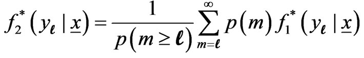 (3.6)
(3.6)
where p(m) is the probability mass function (PMF) of the random variable m and  is the predictive PDF of
  when m is fixed.
Consider the case when m has a truncated Poisson ( ), with PMF
 (3.7)
(3.7)
The predictive PDF and SF of  when m is random can be written as
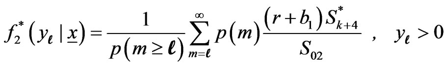 (3.8)
(3.8)
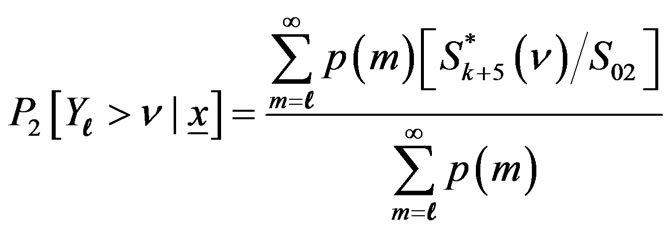 ,(3.9)
where  is given by (3.7),
  and
and  (which are functions of m), are given by (3.3).
4. Application To Exponentiated Burr Type Xii Population
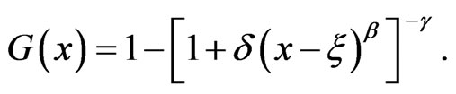
Burr [23] suggested a differential equation of a CDF of a random variable X, whose solution depends on a ‘general’ function of x. Burr chose twelve specific forms for this function to obtain the well-known twelve types of Burr distributions. See Burr [23]. In a different direction, Takahasi [60], compounded the Weibull distribution with the gamma distribution to obtain a 3-parameter Burr XII distribution. Baharith [21], studied the 4-parameter Burr XII (β,g,d,x) whose CDF, for , is of the form
The two-parameter Burr XII (β,g) distribution has CDF and PDF of the form
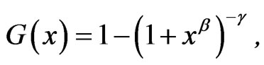 (4.1)
(4.1)
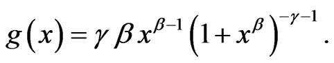 (4.2)
(4.2)
Among the 12 distributions of Burr, the 2-parameter Burr XII (β,g) has found numerous applications. It was proposed as a life time model and its properties were studied by Burr and Cislak [24], Dubey [25,26], Tadikamalla [59] and Lewis [42], among others. Inferences, based on the Burr XII (β,g) distribution and some of its testing measures were made by Papadopoulos [53], Evans and Ragab [31], Lingappaiah [45], Shah and Gekhale [55], AL-Hussaini and Jaheen [12,13]. Khan and Khan [39] and AL-Hussaini [3] characterized the Burr XII (β,g) distribution. Nigm [49] and AL-Hussaini and Jaheen [14] predicted observables based on the Burr XII (β,g) model.
An exponentiated Burr type XII distribution with parameters a,β,g, denoted by EBurr XII(a,β,g), has CDF and PDF of the forms (1.1) and (1.2), where G and g are given by (4.1) and (4.2), respectively. We shall obtain the predictive PDF, and hence predictive bounds of  when the unknown parameters are a,β and g.
Suppose that the baseline distribution G is Burr XII with two unknown parameters β and g. It is assumed that a is independent of (β,g) and that ,
,  and
and , so that the prior PDF of
  is given by

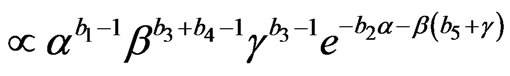 (4.3)
(4.3)
4.1. One-Sample Prediction
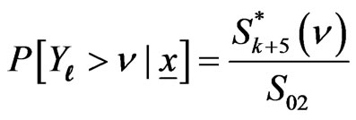
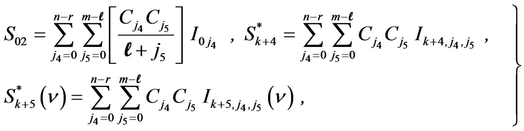
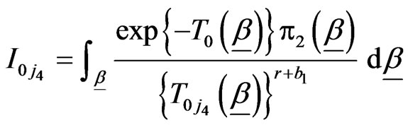
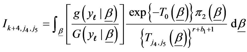
The predictive PDF and SF of  are given, respectively, by
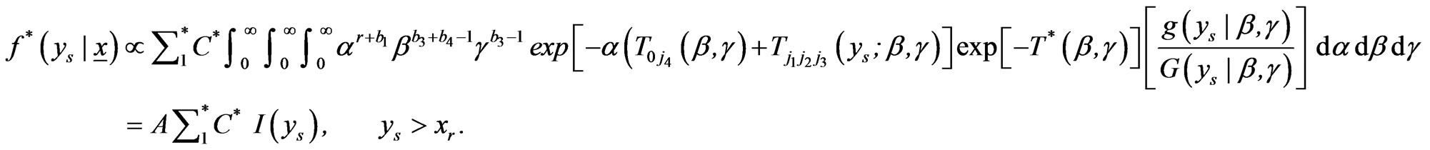
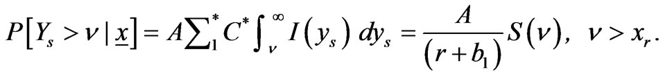
where
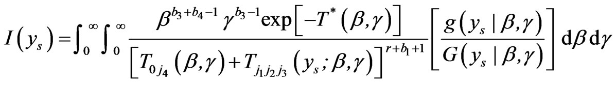
 (4.4)
(4.4)
 ,
, ,
,  and
and  are given, respectively, by (2.5), (2.10), (2.12) and (2.13).
4.2. Two-Sample Prediction
In the following two subsections, it is assumed that the two independent samples of sizes n and m are drawn from an exponentiated population. The size m of the future sample is assumed to be fixed, in subsection 4.2.1 and random in subsection 4.2.2.
4.2.1. Fixed Sample Size
The predictive PDF and SF of the future  are given by
 ,
, where
where
 ,
, ,
, 
 is given by (2.9) ,
 ,
,
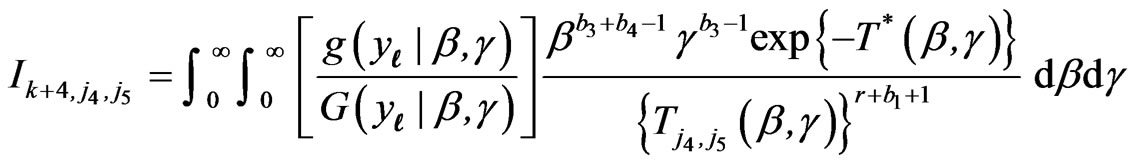

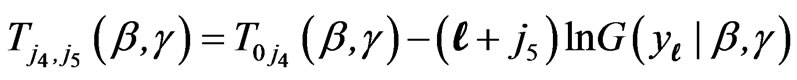
 ,
, ,
, and
and  are given by (2.9), (2.10), (2.12) and (4.4).
A two-sided predictive interval for  is given by
 , where L and U are the solution of (3.5). For proof, see [8].
4.2.2. Random Sample Size
The predictive PDF and SF of the future , when m is random, are given by (3.8) and (3.9), using
  and
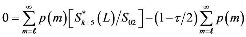
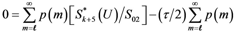
and  defined in section 4.2.1. It follows, from (3.9), that a two-sided predictive interval for
  is given by
 , where L and U are the solution of the two equations
5. Numerical Computations
The numerical examples given here are to illustrate the use of the results obtained.
5.1. Example 1
Twenty observations are generated from the EBurr XII (a = 2.5, β = 1.5, g = 2) according to the expression:
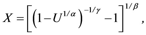 where
where 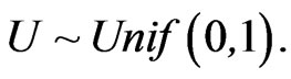
The observations are ordered and only the first 15 out of the 20 observations are assumed to be known. The observations are given as
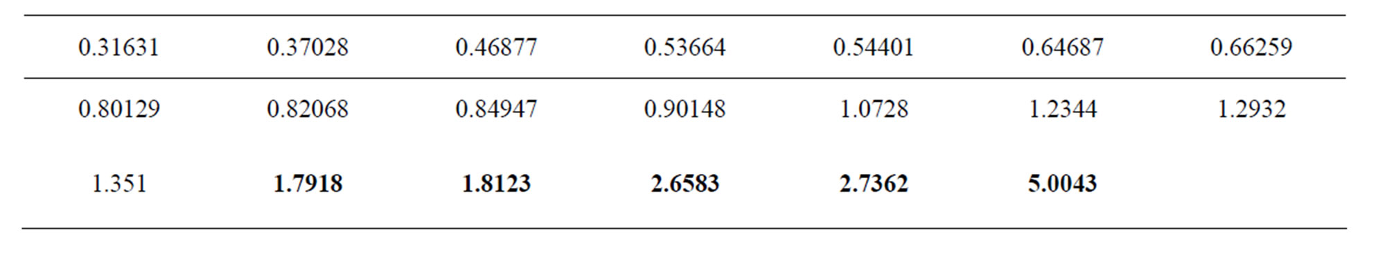
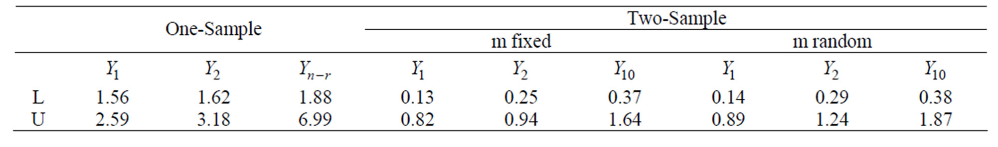
Table 1. Lower and Upper Limits of Some Predicted Values.
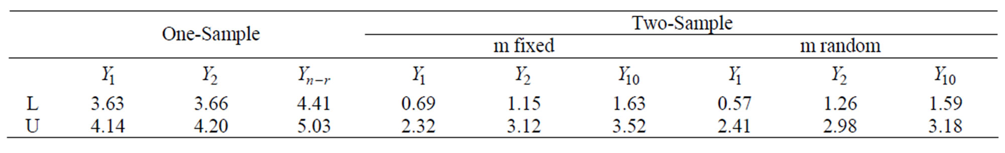
Table 2. Lower and Upper Limits of Some Predicted Values.
When the hyper-parameters are ,
,  ,
,  ,
,  ,
,  , the lower and upper limits for the 95% predictive intervals of
 ,
,  and
and , based on the one-sample scheme, are given in Table 1. On the other hand, when predicti-on is based on the two-sample scheme, Table 1 also shows the lower and upper limits for the 95% predictive intervals of three failure times of a future sample of size m,
  ,
, 
and , of size m, when m is fixed (=10) and when m has a truncated Poisson with
 .
.
5.2. Example 2 (Real Life Data)
The following data (Lawless 2003, p.573, [40]) represent the breaking strength of n = 64 single carbon fibers of length 10, given as ordered1.901, 2.132, 2.203, 2.228, 2.257, 2.350, 2.361, 2.396, 2.397, 2.445, 2.454, 2.454, 2.474, 2.518, 2.522, 2.525, 2.532, 2.575, 2.614, 2.616, 2.618, 2.624, 2.659, 2.675, 2.738, 2.740, 2.856, 2.917, 2.928, 2.937, 2.937, 2.977, 2.996, 3.030, 3.125, 3.139, 3.145, 3.220, 3.223, 3.235, 3.243, 3.264, 3.272, 3.294, 3.332, 3.346, 3.377, 3.408, 3.435, 3.493, 3.501, 3.537, 3.554, 3.562, 3.628, 3.852, 3.871, 3.886, 3.971, 4.024, 4.027, 4.225, 4.395, 5.020.
It is assumed that only 55 (= r) observations are known. AL-Hussaini and Hussein [11], showed that the vector of hyper-parameters (

 ) are appropriate for the prior density of a, β, g so that the EBurr XII distribution fits the set of data using Kolmogorov Smirnov test.
The lower and upper limits for the 95% predictive intervals of ,
,  and
and , are given in Table 2, when based on the one-sample scheme, where n = 64 and r = 55. On the other hand, when prediction is based on the two-sample scheme, with n = 64, r = 55 and m = 10, the lower and upper limits for the 95% predictive intervals of three failure times of a future sample of size m,
  ,
,  and
and , when m is fixed (= 10) and when m has a truncated Poisson with
 , are displayed in Table 2.
6. Concluding Remarks
Bayes 100(1 – t )% predictive interval for future observables is obtained when data are order statistics of a random sample drawn from a population having the exponentiated distribution and only the first r observations are known. The oneand two-sample schemes are used in prediction and a subjective prior is used as the prior belief of the experimenter. In the two-sample case, the Bayes intervals are obtained when the size of the future sample is assumed to be fixed and to be random. In the random case, the size of the future sample follows the Poisson distribution with parameter λ. Results are applied to the exponentiated Burr type XII population. Two examples are given: one uses simulated data and the other uses data representing the breaking strength of 64 single carbon fibers of length 10, found in Lawless [40].
7. References
[1] J.C. Ahuja and S.W. Nash,"The generalized Gompertz-Verhulst family of distributio-ns," Sankhyā, Vol. 29, 1967, pp. 141-161.
[2] E.K. AL-Hussaini,"A Characterization of the Burr type XII distribution," Appl. Math. Lett., Vol. 1, 1991, pp. 59-61.
[3] E.K. AL-Hussaini,"Bayesian prediction under a mixture of two exponential components model based on type I censoring," J. Appl. Statist. Sc. Vol. 8, 1999, pp. 173-185.
[4] E.K. AL-Hussaini, "Prediction: advances and new research," Presented as an invited topical paper in the International Mathematics Conference [Mathematics and the 21st century ], Cairo, Egypt, January 2000.
[5] E.K. AL-Hussaini, On Bayes prediction of future median. Commun. Statist.- Theory Meth., Vol. 30, 2001, pp. 1395-1410.
[6] E.K. AL-Hussaini, "Bayesian predictive density of order statistics based on finite mixture models,". J. Statist. Plann. Inf. Vol. 113, 2003, pp. 15-24.
[7] E.K. AL-Hussaini, "On the exponentiated class of distributions," J. Statist. Theory Appl ., Vol. 9, 2010a, pp. 41-64.
[8] E.K. AL-Hussaini,"Inference based on censored samples from exponentiated populations," Test., Vol. 19, 2010b, pp. 487-513.
[9] E.K. AL-Hussaini and M.A. Gharib,"A new family of distributions as a countable mixture with Poisson added parameter," J. Statist. Theory Appl., Vol. 8, 2009, pp. 169-190.
[10] E.K. AL-Hussaini and M. Ghitany, "On certain countable mixtures of absolutely continuous distributions," Metron,Vol. LXIII, pp. 39-53.
[11] E.K. AL-Hussaini and M. Hussein, "Estimation using censored data from exponentiated Burr type XII distribution," (Submitted).
[12] E.K. AL-Hussaini and Z.F. Jaheen, "Bayes estimation of the parameters, reliability and failure rate functions of the Burr type XII failure model," J. Statist. Comput. Simul.,Vol. 41, 1992, pp. 31- 40.
[13] E.K. AL-Hussaini and Z.F. Jaheen, "Approximate Bayes estimators applied to the Burr model," Commun. Statist.-Theory Meth., Vol. 23, 1994, pp. 99-121.
[14] E.K. AL-Hussaini and Z.F. Jaheen," (1995), Bayes prediction bounds for the Burr type XII failure model," Commun. Statist.-Theory Meth., Vol. 24, 1995. pp. 1829-1842.
[15] E.K. AL-Hussaini and Z.F. Jaheen,"Bayesian prediction bounds for the Burr type XII distribution in the presence of outliers," J. Statist. Plann. Inf., Vol. 55, 1996, pp. 23-37.
[16] E.K. AL-Hussaini and Z.F. Jaheen, "Parametric prediction bounds for the future median of the exponential distribution," Statistics, Vol. 32, 1999, pp. 267 \-275.
[17] E.K. AL-Hussaini, M.A. Mousa and Z.F. Jaheen,"Estimation under the Burr type XII failure model: a comparative study," Test, Vol. 1, 1992. pp. 33-42.
[18] E.K. AL-Hussaini A.M. Nigm and Z.F. Jaheen," Bayesian prediction based on finite mixtures of Lomax components model and type I censoring," Statistics, Vol. 35, 2001, 259-268.
[19] M.A. Ali Mousa and Z.F. Jaheen,"Bayesian prediction for the Burr type XII model based on doubly censored data," Statistics, Vol. 48, 1997, pp. 337-344.
[20] B.C. Arnold and S.J. Press,"Bayesian inference for Pareto populations," J. Economt-rics, Vol. 21, 1983, pp. 287-306.
[21] L.A. Baharith,"On the four-parameter Burr type XII life time model," M.Sc. thesis.King Abdulaziz University, Jeddah, Saudi Arabia, 1997.
[22] J. Bernardo and A. Smith, "Bayesian Theory," Wiley, New York, 1994.
[23] I.W. Burr, "Cumulative frequency functions," Ann. Math. Statist., Vol. 1, 1942, pp. 215-232.
[24] I.W. Burr and P.J. Cislak, (1968)," On a general system of distributions:I. Its curve shaped characteristics; II. The sample median," J. Amer. Statist. Assoc. Vol. 63, 1968, pp. 627-635.
[25] S.D. Dubey,"Statistical contributions to reliability engineerings," ARL TR 72-0155, AD 1774537, 1972.
[26] S.D. Dubey, "Statistical treatment of certain life testing and reliability problems,"ARL TR 73-0155, AD 1774537, 1973.
[27] I. Dunsmore, "The Bayesian predictive distribution in life testing models. Technom-trics Vol. 16, 1974, pp. 455-460.
[28] I.G. Evans and A.M. Nigm, "Bayesian prediction for two-parameter Weibull lifetime model," Commun. Statist.-Theory Meth., Vol. 9, 1980a, pp. 649-658.
[29] I.G. Evans and A.M. Nigm, "Bayesian 1-sample prediction for the 2-parameter Wei-bull distribution," IEEE Trans. Rel., Vol. R-29, 1980b, pp. 410-413.
[30] I.G. Evans and A.M. Nigm,"Bayesian prediction for the left truncated exponential distribution," Technometrics 22, 1980c, pp. 201-204.
[31] I.G. Evans and A.S. Ragab, "Bayesian inferences given a type-2 censored sample from Burr distribution," Commun. Statist.-Theory Meth.,Vol. 12, 1983, pp. 1569-1580.
[32] S. Geisser, "Predicting Pareto and exponential observables," Canad. J. Statist. Vol. 12, 1984, pp. 143-152.
[33] S. Geisser,"Prediction Inference: An Introduction," Chapman and Hall, London, 1993.
[34] R.C. Gupta and R.D. Gupta,"On the distribution of order statistics for a random sample size," Statist. Neelandica. Vol. 38 , 1984, pp. 13-19.
[35] R.C. Gupta and R.D. Gupta, "Proportional reversed hazard rate model and its applications," J. Statist. Plann. Inf., Vol. 137 , 2007, pp. 3525-3536.
[36] H.A. Howlader, HPD prediction intervals for Rayleigh distribution," IEEE Trans. Rel., Vol. 34, 1985, pp. 121-123.
[37] Z.F. Jaheen,"Bayesian estimations and predictions based on single Burr type XII models and their finite mixture," Ph.D. dissertation, University of Assiut, Egypt, 1993.
[38] K. Kaminsky and P. Nelson, "Prediction of order statistics," In Balakrishnan, N. and Rao, C.R. Eds. Handbook of Statistics, vol.17, Elsevier Science, Amesterdam, The Netherland, 1998, pp. 431-450.
[39] A.H. Khan and A.I. Khan, "Moments of order statistics from Burr's distribution and its characterization," Metron, Vol. 45, 1987, pp. 21-29.
[40] J.F. Lawless,"Statistical Models and Methods for Lifetime Data," 2nd ed, Wiley, 2003.
[41] E.L. Lehmann,"The power of rank tests," Ann. Math. Statist. 24,1953, pp. 28-43.
[42] A.W. Lewis, The Burr distribution as a general parametric family in survivorship and reliability theory applications. Ph.D. thesis, University of North Carolina, 1981.
[43] T. Lwin,"Estimating the tale of the Paretian law," Scand. Actuar. J. Vol. 55, 1972, pp. 170-178.
[44] G.S. Lingappaiah,"Bayesian approach to prediction and the spacings in the exponential distribution," Ann. Instit. Statist. Math., Vol. 31, 1979, pp. 391-401.
[45] G.S. Lingappaiah,"Bayesian approach to the estimation of parameters in the Burr's XII distribution with outliers," J. Orissa Math. Soc., Vol. 1, 1983. pp. 55-59.
[46] H.J. Malik,"Bayesian estimation of the Paretian index. Scand. Actuar. J., Vol. 53, 1970, pp. 6-9.
[47] A.W. Marshall and I. Olkin,"A new method for adding a parameter to a family of distributions with applications to the exponential and Weibull families," Biometrika Vol. 84 1997, pp. 641 -652.
[48] H.N. Nagaraja,"Prediction problems," In: Balackrishnan, N. and Basu, A.P., Eds., The exponential distribution: theory and applications, Gordon and Breach, New York, 1995, pp.139-163.
[49] A.M Nigm, "Prediction bounds for the Burr model," Commun. Statist.-Theory Meth., Vol. 17, 1988, pp. 287- 296.
[50] A.M. Nigm, and H.I. Hamdy, "Bayesian prediction bounds for the Pareto lifetime," Commun. Statist.-Theory Meth., Vol. 16, 1987, pp. 1761-1772.
[51] A.M. Nigm, E.K. AL-Hussaini, and Z.F. Jaheen,"Bayesian two-sample prediction under the Lomax model with fixed and random sample size. J. Appl. Statist. Sc., Vol. 15, 2007, pp. 381-390.
[52] J.K. Patel,"Prediction intervals-a review," Commun. Statist.-Theory Meth., Vol. 18, 1989, pp. 2393-2465.
[53] A.S. Papadopoulos,"The Burr distribution as a life time model from a Bayesian approach," IEEE Trans. Rel., Vol. R-27, 1978, pp. 369-371.
[54] M.Z. Raqab,"Predictors of future order statistics from type II censoring samples," Ph.D. dissertation, Ohio State University, Colombus, 1992.
[55] A. Shah and D.V. Gokhale, "On maximum product of spacings (MPS) estimation for Burr XII distribution,"Commun. Statist.-Theory Meth. Vol. 22, 1993, pp. 615-641.
[56] S.K. Sinha, "On the prediction limits for Rayleigh life distribution," Culcutta. Statist. Assoc. Bulletin Vol. 39, 1990, pp. 104-109.
[57] S.K. Sinha, and H.A. Howlader,"On the sampling of the Bayes estimators of the Pareto parameter with proper and improper priors and associated goodness of fit. Tech. Report No. 103. Dept. Statist., university of Mintoba, Winnipeg, Canada, 1980
[58] S.K. Sinha, and H.A. Howlader, Credible and HPD intervals of the parameter and reliability of Rayleigh distribution. IEEE Trans. Rel., Vol. 32, 1983, pp. 217-220.
[59] Tadikamalla, P.R. (1980). A look at the Burr and related distributions. Inter. Statist. Review, Vol. 48, 1980, pp. 337-344.
[60] K. Takahasi,"Note on the multivariate Burr's distribution," Ann. Instit. Statist. Math.1965, Vol. 17, 1965, pp. 257 -260.
[61] P.F. Verhulst, "Notice sur la loi population dans son accroissement," Correspondan-ce mathématique et physique, publiée par L.A.L. Quetelet, Vol. 10, 1838, pp. 113-121.
[62] P.F. Verhulst, "Recheches mathématiques sur la loi d'accroissement de la populati-on," Nouvelle mémoire de l'Academie Royale de Sciences et Belle-Lettres de Bruxelles [i.e. Mémoire Series 2], Vol. 18, 1845, pp. 1-42.
[63] P.F. Verhulst, "Deuxiéme mémoire sur la loi d'accroissment de la population," Mé-moire de l'Academie Royale des Sciences, des Lettres et de Beaux-Arts de Belgique, Seri-es 2, Vol. 20, 1847, pp. 1-32.
[64] A. Zellner, "An Introduction to Bayesian Inference in Econometrics," Wiley, 1971.