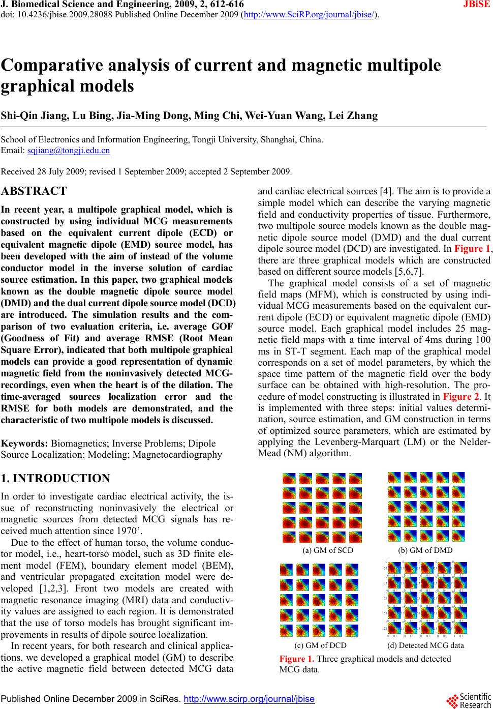J. Biomedical Science and Engineering, 2009, 2, 612-616 JBiSE
doi: 10.4236/jbise.2009.28088 Published Online December 2009 (http://www.SciRP.org/journal/jbise/ ).
Published Online December 2009 in SciRes. http://www.scirp.org/journal/jbise
Comparative analysis of current and magnetic multipole
graphical models
Shi-Qin Jiang, Lu Bing, Jia-Ming Dong, Ming Chi, Wei-Yuan Wang, Lei Zhang
School of Electronics and Information Engineering, Tongji University, Shanghai, China.
Received 28 July 2009; revised 1 September 2009; accepted 2 September 2009.
ABSTRACT
In recent year, a multipole graphical model, which is
constructed by using individual MCG measurements
based on the equivalent current dipole (ECD) or
equivalent magnetic dipole (EMD) source model, has
been developed with the aim of instead of the volume
conductor model in the inverse solution of cardiac
source estimation. In this paper, two graphical models
known as the double magnetic dipole source model
(DMD) and the dual current dipole source model (DCD)
are introduced. The simulation results and the com-
parison of two evaluation criteria, i.e. average GOF
(Goodness of Fit) and average RMSE (Root Mean
Square Error), indicated that both multipole graphical
models can provide a good representation of dynamic
magnetic field from the noninvasively detected MCG-
recordings, even when the heart is of the dilation. The
time-averaged sources localization error and the
RMSE for both models are demonstrated, and the
characteristic of two multipole models is discussed.
Keywords: Biomagnetics; Inverse Problems; Dipole
Source Localization; Modeling; Magnetocardiography
1. INTRODUCTION
In order to investigate cardiac electrical activity, the is-
sue of reconstructing noninvasively the electrical or
magnetic sources from detected MCG signals has re-
ceived much attention since 1970’.
Due to the effect of human torso, the volume conduc-
tor model, i.e., heart-torso model, such as 3D finite ele-
ment model (FEM), boundary element model (BEM),
and ventricular propagated excitation model were de-
veloped [1,2,3]. Front two models are created with
magnetic resonance imaging (MRI) data and conductiv-
ity values are assigned to each region. It is demonstrated
that the use of torso models has brought significant im-
provements in results of dipole source localization.
In recent years, for both research and clinical applica-
tions, we developed a graphical model (GM) to describe
the active magnetic field between detected MCG data
and cardiac electrical sources [4]. The aim is to provide a
simple model which can describe the varying magnetic
field and conductivity properties of tissue. Furthermore,
two multipole source models known as the double mag-
netic dipole source model (DMD) and the dual current
dipole source model (DCD) are investigated. In Figure 1,
there are three graphical models which are constructed
based on different source models [5,6,7].
The graphical model consists of a set of magnetic
field maps (MFM), which is constructed by using indi-
vidual MCG measurements based on the equivalent cur-
rent dipole (ECD) or equivalent magnetic dipole (EMD)
source model. Each graphical model includes 25 mag-
netic field maps with a time interval of 4ms during 100
ms in ST-T segment. Each map of the graphical model
corresponds on a set of model parameters, by which the
space time pattern of the magnetic field over the body
surface can be obtained with high-resolution. The pro-
cedure of model constructing is illustrated in Figure 2. It
is implemented with three steps: initial values determi-
nation, source estimation, and GM construction in terms
of optimized source parameters, which are estimated by
applying the Levenberg-Marquart (LM) or the Nelder-
Mead (NM) algorithm.
(a) GM of SCD (b) GM of DMD
(c) GM of DCD (d) Detected MCG data
Figure 1. Three graphical models and detected
MCG data.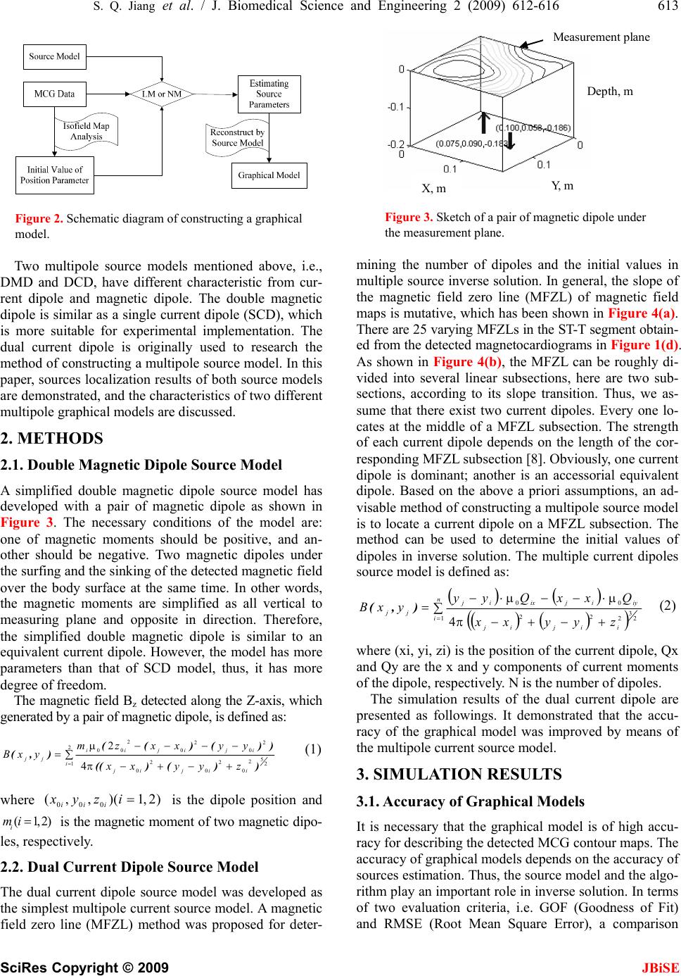

S. Q. Jiang et al. / J. Biomedical Science and Engineering 2 (2009) 612-616 613
SciRes Copyright © 2009 JBiSE
Figure 2. Schematic diagram of constructing a graphical
model.
Two multipole source models mentioned above, i.e.,
DMD and DCD, have different characteristic from cur-
rent dipole and magnetic dipole. The double magnetic
dipole is similar as a single current dipole (SCD), which
is more suitable for experimental implementation. The
dual current dipole is originally used to research the
method of constructing a multipole source model. In this
paper, sources localization results of both source models
are demonstrated, and the characteristics of two different
multipole graphical models are discussed.
2. METHODS
2.1. Double Magnetic Dipole Source Model
A simplified double magnetic dipole source model has
developed with a pair of magnetic dipole as shown in
Figure 3. The necessary conditions of the model are:
one of magnetic moments should be positive, and an-
other should be negative. Two magnetic dipoles under
the surfing and the sinking of the detected magnetic field
over the body surface at the same time. In other words,
the magnetic moments are simplified as all vertical to
measuring plane and opposite in direction. Therefore,
the simplified double magnetic dipole is similar to an
equivalent current dipole. However, the model has more
parameters than that of SCD model, thus, it has more
degree of freedom.
The magnetic field Bz detected along the Z-axis, which
generated by a pair of magnetic dipole, is defined as:
∑+−+−
−−−−
==
2
12
5
2
0
2
0
2
0
2
0
2
0
2
00
4
2
iiijij
ijijii
jj zyyxx
yyxxzm
yxB ))()((
))()((
),(π
µ (1)
where 000
(,,)(1,2)
iii
xyzi= is the dipole position and
(1,2)
i
mi= is the magnetic moment of two magnetic dipo-
les, respectively.
2.2. Dual Current Dipole Source Model
The dual current dipole source model was developed as
the simplest multipole current source model. A magnetic
field zero line (MFZL) method was proposed for deter-
M
easurement plane
Depth, m
X, m Y, m
Figure 3. Sketch of a pair of magnetic dipole under
the measurement plane.
mining the number of dipoles and the initial values in
multiple source inverse solution. In general, the slope of
the magnetic field zero line (MFZL) of magnetic field
maps is mutative, which has been shown in Figure 4(a).
There are 25 varying MFZLs in the ST-T segment obtain-
ed from the detected magnetocardiograms in Figure 1(d).
As shown in Figure 4(b), the MFZL can be roughly di-
vided into several linear subsections, here are two sub-
sections, according to its slope transition. Thus, we as-
sume that there exist two current dipoles. Every one lo-
cates at the middle of a MFZL subsection. The strength
of each current dipole depends on the length of the cor-
responding MFZL subsection [8]. Obviously, one current
dipole is dominant; another is an accessorial equivalent
dipole. Based on the above a priori assumptions, an ad-
visable method of constructing a multipole source model
is to locate a current dipole on a MFZL subsection. The
method can be used to determine the initial values of
dipoles in inverse solution. The multiple current dipoles
source model is defined as:
(
)
(
)
() () ( )
∑+−+−
⋅−−⋅−
=
=
n
i
iijij
iyijixij
jj zyyxx
QxxQyy
yxB 12
3
2
22
00
4π
µµ
),( (2)
where (xi, yi, zi) is the position of the current dipole, Qx
and Qy are the x and y components of current moments
of the dipole, respectively. N is the number of dipoles.
The simulation results of the dual current dipole are
presented as followings. It demonstrated that the accu-
racy of the graphical model was improved by means of
the multipole current source model.
3. SIMULATION RESULTS
3.1. Accuracy of Graphical Models
It is necessary that the graphical model is of high accu-
racy for describing the detected MCG contour maps. The
accuracy of graphical models depends on the accuracy of
sources estimation. Thus, the source model and the algo-
rithm play an important role in inverse solution. In terms
of two evaluation criteria, i.e. GOF (Goodness of Fit)
and RMSE (Root Mean Square Error), a comparison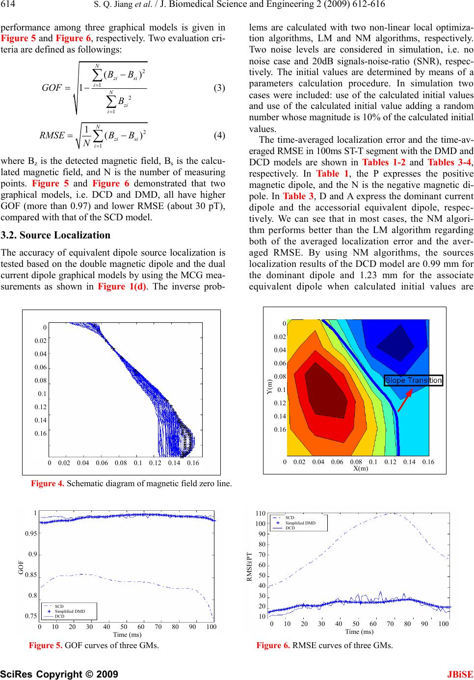

614 S. Q. Jiang et al. / J. Biomedical Science and Engineering 2 (2009) 612-616
SciRes Copyright © 2009 JBiSE
performance among three graphical models is given in
Figure 5 and Figure 6, respectively. Two evaluation cri-
teria are defined as followings:
2
1
2
1
()
1
N
zisi
iN
zi
i
BB
GOF
B
=
=
−
=−
∑
∑ (3)
2
1
1
()
N
zisi
i
RMSEBB
N
=
=−
∑ (4)
where Bz is the detected magnetic field, Bs is the calcu-
lated magnetic field, and N is the number of measuring
points. Figure 5 and Figure 6 demonstrated that two
graphical models, i.e. DCD and DMD, all have higher
GOF (more than 0.97) and lower RMSE (about 30 pT),
compared with that of the SCD model.
3.2. Source Localization
The accuracy of equivalent dipole source localization is
tested based on the double magnetic dipole and the dual
current dipole graphical models by using the MCG mea-
surements as shown in Figure 1(d). The inverse prob-
lems are calculated with two non-linear local optimiza-
tion algorithms, LM and NM algorithms, respectively.
Two noise levels are considered in simulation, i.e. no
noise case and 20dB signals-noise-ratio (SNR), respec-
tively. The initial values are determined by means of a
parameters calculation procedure. In simulation two
cases were included: use of the calculated initial values
and use of the calculated initial value adding a random
number whose magnitude is 10% of the calculated initial
values.
The time-averaged localization error and the time-av-
eraged RMSE in 100ms ST-T segment with the DMD and
DCD models are shown in Tables 1-2 and Tables 3-4,
respectively. In Table 1, the P expresses the positive
magnetic dipole, and the N is the negative magnetic di-
pole. In Table 3, D and A express the dominant current
dipole and the accessorial equivalent dipole, respec-
tively. We can see that in most cases, the NM algori-
thm performs better than the LM algorithm regarding
both of the averaged localization error and the aver-
aged RMSE. By using NM algorithms, the sources
localization results of the DCD model are 0.99 mm for
the dominant dipole and 1.23 mm for the associate
equivalent dipole when calculated initial values are
(a) MFZLs in ST-T segment (b) Slope variation of the MFZL
Figure 4. Schematic diagram of magnetic field zero line.
Figure 5. GOF curves of three GMs. Figure 6. RMSE curves of three GMs.
0 0.02 0.04 0.06 0.08 0.1 0.12 0.14 0.16
0
0.02
0.04
0.06
0.08
0.1
0.12
0.14
0.16
0
0.02
0.04
0.06
0.08
0.1
0.12
0.14
0.16
Y(m)
0 0.02 0.04 0.06 0.08 0.1 0.12 0.14 0.16
X(m)
0 10 20 30 40 50 60 70 80 90 100
Time (ms)
SCD
Simplified DMD
DCD
1
0.95
0.9
0.85
0.8
0.75
GOF
RMSE(PT
)
110
100
90
80
70
60
50
40
30
20
10 0 10 20 30 40 50 60 70 80 90 100
Time (ms)
SCD
Simplified DMD
DCD

S. Q. Jiang et al. / J. Biomedical Science and Engineering 2 (2009) 612-616 615
SciRes Copyright © 2009 JBiSE
Table 1. Averaged localization error of DMD model (mm).
Calculated Initial Values 10% Random
Initial
values
Data
noises LM NM LM NM
No
noise P N
0.0
0.0 0.0 0.0 0.34 0.69 0.41 1.06
20db
noise P N
1.34
3.69 1.86 4.84 1.39 3.74 1.40 3.72
Table 2. Averaged RMSE of DMD model (pt).
Calculated Initial Values 10% Random
Initial
values
Data
noises LM NM LM
NM
No noise 0.0 0.0 189 155
20db noise 232 187 255 196
Table 3. Averaged localization error of DCD model (mm).
Calculated Initial Values 10% Random
Initial
vaues
Data
noises LM NM LM NM
No
noise
D
A
20db
noise
D
A
0.0
0.0
1.20
1.79
0.0
0.00
0.99
1.22
1.14
1.43
1.71
1.88
0.89
0.96
0.99
1.23
Table 4. Averaged RMSE of DCD model (PT).
Calculated Initial Values 10% Random
Initial
values
Data
noises LM NM LM NM
No noise
20db noise
0.0
228
0.0
137
211
236
112
155
used. In despite of the localization results of the DMD
model have been improved, but they are still not as
good as that of the DCD model.
Furthermore, Figure 7 to Figure 8 show the time-
varying position and orientation curves of two magnetic
dipoles in the 100 ms ST-T segment. The positive mag-
netic dipole, i.e. the dipole under the surfing of the mag-
netic field contour map, moved in a range of 0.11-0.12 m
at Z direction, and the negative dipole moved in a dis-
tance about 0.106-0.116 m away from the measurement
plane on the chest. In other words, the depth of two equi-
valent magnetic dipoles changed in a small region. Two
moving magnetic dipoles are confined within the region
of the heart. It is noticeable that x, y, z components cur-
ves of the location of two equivalent current dipoles are
shown in Figure 9 and Figure 10. The first current di-
pole, i.e. the dominant dipole, moved in a range of 0.06-
0.07 m at Z direction, and the accessorial equivalent
dipole, moved in a distance of 0.11-0.14 m away from
the measurement plane on the chest. In other words, the
accessorial equivalent dipole located a little deeper than
the dominant dipole. Two moving current dipoles are
confined within the region of the heart.
In sum, two equivalent magnetic dipoles are moved in
almost the same depth as the accessorial equivalent cur-
rent dipole. The x and y components curves of the loca-
tion of the accessorial equivalent current dipole have
obvious sudden variation, however, two equivalent mag-
netic dipoles have no such phenomena.
4. CONCLUSIONS
Two multipole graphical models are introduced for the
investigation of the cardiac electrical activity in this paper.
Because the accuracy of graphical models depends on the
accuracy of sources estimation, thus, the initial value
010 2030405060 708090100
0.05
0.06
0.07
0.08
0.09
0.1
0.11
0.12
Time(ms)
Location(m)
Location in x
Location in y
Location in z
Figure 7. The time-varying location curves of the positive
magnetic dipole.
010 20304050 60 70 8090 100
0.04
0.05
0.06
0.07
0.08
0.09
0.1
0.11
0.12
0.13
Time(ms)
Location(m)
Location in x
Location in y
Location in z
Figure 8. The time-varying location curves of the negative
magnetic dipole.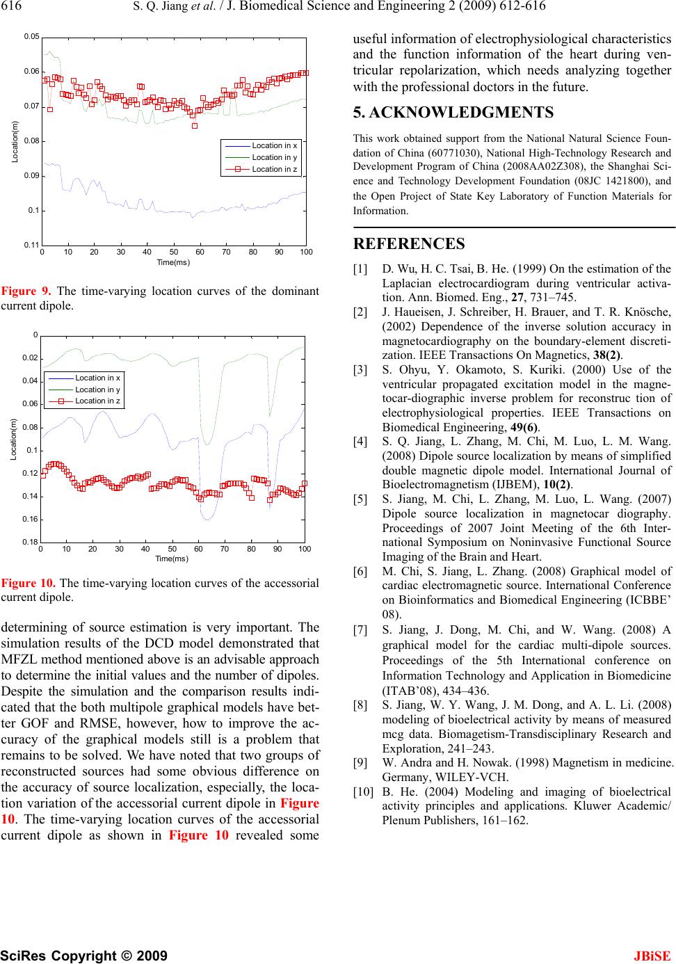

616 S. Q. Jiang et al. / J. Biomedical Science and Engineering 2 (2009) 612-616
SciRes Copyright © 2009 JBiSE
010 2030 40 506070 80 90100
0.05
0.06
0.07
0.08
0.09
0.1
0.11
Time(ms)
Location(m)
Location in x
Location in y
Location in z
Figure 9. The time-varying location curves of the dominant
current dipole.
010 2030 4050 60 7080 90100
0
0.02
0.04
0.06
0.08
0.1
0.12
0.14
0.16
0.18
Time(ms)
Location(m)
Location in x
Location in y
Location in z
Figure 10. The time-varying location curves of the accessorial
current dipole.
determining of source estimation is very important. The
simulation results of the DCD model demonstrated that
MFZL method mentioned above is an advisable approach
to determine the initial values and the number of dipoles.
Despite the simulation and the comparison results indi-
cated that the both multipole graphical models have bet-
ter GOF and RMSE, however, how to improve the ac-
curacy of the graphical models still is a problem that
remains to be solved. We have noted that two groups of
reconstructed sources had some obvious difference on
the accuracy of source localization, especially, the loca-
tion variation of the accessorial current dipole in Figure
10. The time-varying location curves of the accessorial
current dipole as shown in Figure 10 revealed some
useful information of electrophysiological characteristics
and the function information of the heart during ven-
tricular repolarization, which needs analyzing together
with the professional doctors in the future.
5. ACKNOWLEDGMENTS
This work obtained support from the National Natural Science Foun-
dation of China (60771030), National High-Technology Research and
Development Program of China (2008AA02Z308), the Shanghai Sci-
ence and Technology Development Foundation (08JC 1421800), and
the Open Project of State Key Laboratory of Function Materials for
Information.
REFERENCES
[1] D. Wu, H. C. Tsai, B. He. (1999) On the estimation of the
Laplacian electrocardiogram during ventricular activa-
tion. Ann. Biomed. Eng., 27, 731–745.
[2] J. Haueisen, J. Schreiber, H. Brauer, and T. R. Knösche,
(2002) Dependence of the inverse solution accuracy in
magnetocardiography on the boundary-element discreti-
zation. IEEE Transactions On Magnetics, 38(2).
[3] S. Ohyu, Y. Okamoto, S. Kuriki. (2000) Use of the
ventricular propagated excitation model in the magne-
tocar-diographic inverse problem for reconstruc tion of
electrophysiological properties. IEEE Transactions on
Biomedical Engineering, 49(6).
[4] S. Q. Jiang, L. Zhang, M. Chi, M. Luo, L. M. Wang.
(2008) Dipole source localization by means of simplified
double magnetic dipole model. International Journal of
Bioelectromagnetism (IJBEM), 10(2).
[5] S. Jiang, M. Chi, L. Zhang, M. Luo, L. Wang. (2007)
Dipole source localization in magnetocar diography.
Proceedings of 2007 Joint Meeting of the 6th Inter-
national Symposium on Noninvasive Functional Source
Imaging of the Brain and Heart.
[6] M. Chi, S. Jiang, L. Zhang. (2008) Graphical model of
cardiac electromagnetic source. International Conference
on Bioinformatics and Biomedical Engineering (ICBBE’
08).
[7] S. Jiang, J. Dong, M. Chi, and W. Wang. (2008) A
graphical model for the cardiac multi-dipole sources.
Proceedings of the 5th International conference on
Information Technology and Application in Biomedicine
(ITAB’08), 434–436.
[8] S. Jiang, W. Y. Wang, J. M. Dong, and A. L. Li. (2008)
modeling of bioelectrical activity by means of measured
mcg data. Biomagetism-Transdisciplinary Research and
Exploration, 241–243.
[9] W. Andra and H. Nowak. (1998) Magnetism in medicine.
Germany, WILEY-VCH.
[10] B. He. (2004) Modeling and imaging of bioelectrical
activity principles and applications. Kluwer Academic/
Plenum Publishers, 161–162.