Paper Menu >>
Journal Menu >>
 J. Biomedical Science and Engineering, 2009, 2, 587-593 doi: 10.4236/jbise.2009.28085 Published Online December 2009 (http://www.SciRP.org/journal/jbise/ JBiSE ). Published Online December 2009 in SciRes. http://www.scirp.org/journal/jbise Fitting evolutionary process of matrix protein 2 family from influenza A virus using analytical solution of differential equation Shao-Min Yan1, Zhen-Chong Li1, Guang Wu2* 1National Engineering Research Center for Non-food Biorefinery, Guangxi Academy of Sciences, 98 Daling Road, Nanning, Guangxi, China; 2Computational Mutation Project, DreamSciTech Consulting, 301, Building 12, Nanyou A-zone, Jiannan Road, Shenzhen, Guang- dong, China. Email: hongguanglishibahao@yahoo.com Received 22 August 2009; revised 3 September 2009; accepted 4 September 2009. ABSTRACT The evolution of protein family is a process along the time course, thus any mathematical methods that can describe a process over time could be possible to de- scribe an evolutionary process. In our previously con- cept-initiated study, we attempted to use the differen- tial equation to describe the evolution of hemaggluti- nins from influenza A viruses, and to discuss various issues related to the building of differential equation. In this study, we attempted not only to use the dif- ferential equation to describe the evolution of matrix protein 2 family from influenza A virus, but also to use the analytical solution to fit its evolutionary process. The results showed that the fitting was pos- sible and workable. The fitted model parameters provided a way to further determine the evolutionary dynamics and kinetics, a way to more precisely pre- dict the time of occurrence of mutation, and a way to figure out the interaction between protein family and its environment. Keywords: Amino-Acid Pair Predictability; Differential Equation; Evolution; Fitting; Influenza A Virus; Matrix Protein 2 1. INTRODUCTION Very recently, we explored the possibility to use a dif- ferential equation to describe the evolution of hemagglu- tinin proteins from influenza A virus [1]. However, there are ten types of proteins from influ- enza A viruses, it is necessary to explore whether or not this differential description can be applied to other pro- teins from influenza A viruses. Also, it is intriguing to use the analytic solution of differential equation to fit the evolution of proteins from influenza A viruses. This is so, because the mathematical modeling is gen- erally the ending point of empiric experiments, and more importantly the mathematical modeling can provide us the tool for predicting the future of evolution. As the evolution is a process along the time course, we at first needed to represent an evolutionary subject along the time course, and then we could consider how to apply the mathematical modeling to this process. Now we are particularly interested in the evolution of proteins. However, a protein generally is a sequence of letters, which represent amino acids. Thus we need a method to represent a protein family along the time course before modeling [2-5]. In general, the evolution is a process of exchanging substances between a living subject and its environment. In this context, the differential equation is quite suitable because we defined outputinput d t dy for exchang- ing substance between a protein family and its environ- ment along the time course [1]. As we know that the evolution of proteins goes through mutations, which bring in new mutating amino acids and take out mutated amino acids. This again re- quires the conversion of amino acids into numbers to represent the exchange [2-5]. Among ten types of proteins from influenza A virus, the matrix protein 2 (M2) is important because it con- structs a proton channel in the virion and it is essential for infection [6]. Thus, the M2 protein was the target for anti-influenza drugs, and the M2 ion channel blockers was approved to treat influenza virus infections [7,8], but their use is limited by high frequencies of the resis- tance among currently circulating strains [9,10]. Also, a vaccine was designed basing on the conserved ectodo- main of M2 protein, which could match multiple influ- enza virus strains including multiple subtypes [11]. In this study, our effort was made to apply the differ- ential description to the evolution of M2 protein family from influenza A virus, and to use the analytical solution of differential equations to fit the evolutionary process of  588 S. M. Yan et al. / J. Biomedical Science and Engineering 2 (2009) 587-593 SciRes Copyright © 2009 IALS AND METHODS 2 proteins of influenza A virus sampled ers ins into ABF- 01 acids (E) and 11 le BF01755 M2 pr cession number ABF- 01 bove computation, the difference in pr tial Equation 2 proteins would have a JBiSE M2 proteins. 2. MATER 2.1. Data 5926 full-length M from 1959 to 2008 were obtained from the influenza virus resources [12]. After excluded identical sequences, 1084 M2 proteins were actually used in this study. 2.2. Conversion of Proteins into Numb For two purposes, we needed to convert M2 prote numbers: 1) we needed a single number for a single M2 protein so that we could present the evolution of M2 protein family over time, and 2) we needed a number to present mutation, which resulted in numerical exchange between M2 protein and its environment. We used the amino-acid pair predictability to do this job [2-5]. For example, an M2 protein (accession number 755) from an avian influenza virus, strain A/chi- cken/Magetan/BBVW/2005(H5N1), had 97 amino acids. The first and second amino acids could be counted as an amino-acid pair, the second and third as another amino- acid pair, the third and fourth, until the 96th and 97th, thus there were 96 amino-acid pairs. This M2 protein had 10 glutamic ucines (L): if the permutation could predict the ap- pearance of amino-acid pair EL, it would appear once (10/9711/9696=1.13); actually it did appear once, so the pair EL was predictable. By contrast, this M2 protein had 7 isoleucines (I): if the permutation could predict the appearance of amino-acid pair IL, it would appear once (7/9711/9696=0.79); however, it appeared three times in realty, so the pair IL was unpredictable. In this way, all amino-acid pairs in A otein were classified as predictable and unpredictable, which were 17.71% and 82.29%. Taking another M2 protein (ac 771) as example, this M2 protein had only one amino acid different from ABF01755 M2 protein at position 65. However, its predictable and unpredictable portions were 20.83% and 79.17%. Thus, the amino-acid pair predict- ability distinguished the difference between M2 proteins in numbers rather than in letters that represented amino acids in proteins. Based on the a edictable portion between ABF01755 and ABF01771 M2 proteins was −3.12% (17.71%−20.83%), which was regarded as the exchange between M2 protein and its environment. 2.3. Differen If ABF01755 and ABF01771 M direct relation due to a single mutation, the difference between them was outputinput dy , where y was the difference in prede time re- quired for mutation, input was the predictable portion brought in by mutating amino acid, output was the pre- dictable portion taken away by mutated amino acid. Unfortunately, we had no way to know if ABF01 dt icable portion, t was th 755 an sing the pe est and Mann-Whitney U-test were used 3. RESULTS AND DISCUSSION utation rela- d ABF01771 M2 proteins had a direct mutation rela- tionship although both were sampled in 2005. As the predictable portion was determined u rmutation based on random principle, thus this ex- change was in fact the exchange of randomness between M2 proteins and their environment, more accurately was the exchange of entropy between M2 proteins and their environment [1]. 2.4. Statistics The Student’s t-t to compare the difference between uphill and downhill half-life, and P<0.05 was considered statistically sig- nificant. The SigmaPlot for Windows was used for fit- ting [13]. Ideally, we would hope to have a direct m tionship for all 1084 M2 proteins from 1959 to 2008 involved in this study, because then we would have outputinput d t dy for each mutation relationship be- M2 proteins. Although it was impossible to fi tween any related two nd out such a rela- tio hand, our computations on predictable po Figure 1 presented th al Solution ted that the possi- nship among all of these M2 proteins sampled every- where in the world, the real mutation relationship worked in this way no matter if we had sampled them or not. Thus, we had a system of differential equations for all M2 proteins. On the other rtions of 1084 M2 proteins provided us with the most update evolutionary process in Figure 1, which was read as follows. For example, the solid curve in the top panel presented the evolution of 1084 M2 proteins from 1959 to 2008, and each point was the mean value of predict- able portions of all M2 proteins in given year with its standard deviation (vertically grey line). The similar reading was applied to other panels. So the fluctuating solid curves in e evolutionary process over time. If we could use the differential equation to describe these solid curves, it would mean that we were able to model the evolutionary process of M2 proteins. 3.1. Possibly Analytic These fluctuating solid curves sugges 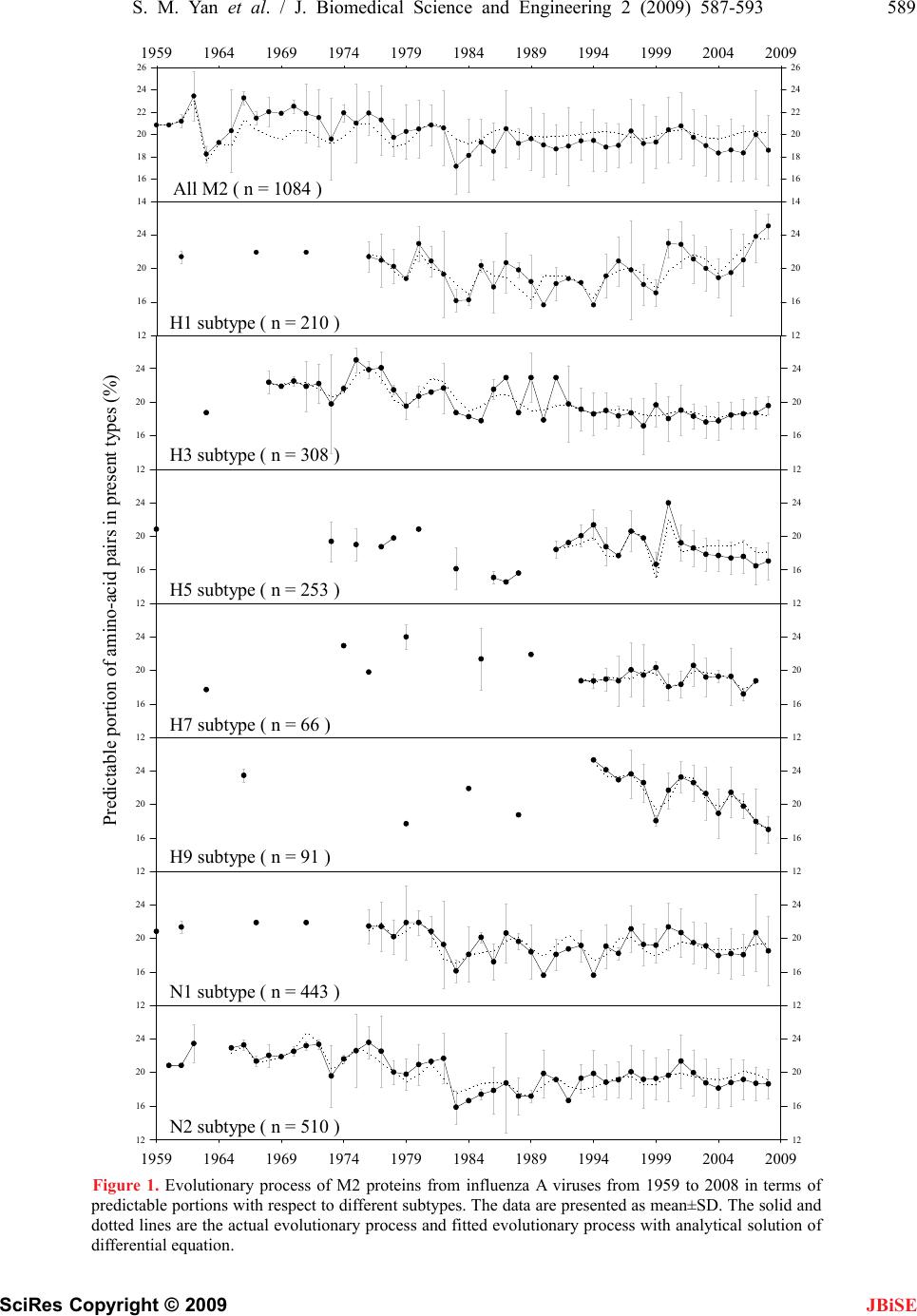 S. M. Yan et al. / J. Biomedical Science and Engineering 2 (2009) 587-593 589 SciRes Copyright © 2009 12 16 20 24 12 16 20 24 12 16 20 24 12 16 20 24 Predictable portion of amino-acid pairs in present types (%) 12 16 20 24 12 16 20 24 12 16 20 24 12 16 20 24 12 16 20 24 12 16 20 24 H1 subtype ( n = 210 ) H3 subtype ( n = 308 ) H5 subtype ( n = 253 ) H7 subtype ( n = 66 ) H9 subtype ( n = 91 ) 12 16 20 24 12 16 20 24 1959 1964 1969 1974 1979 1984 1989 1994 1999 2004 2009 12 16 20 24 12 16 20 24 N2 subtype ( n = 510 ) N1 subtype ( n = 443 ) 1959 1964 1969 1974 1979 1984 1989 1994 1999 2004 2009 14 16 18 20 22 24 26 14 16 18 20 22 24 26 All M2 ( n = 1084 ) Figure 1. Evolutionary process of M2 proteins from influenza A viruses from 1959 to 2008 in terms of predictable portions with respect to different subtypes. The data are presented as mean±SD. The solid and dotted lines are the actual evolutionary process and fitted evolutionary process with analytical solution of differential equation. JBiSE 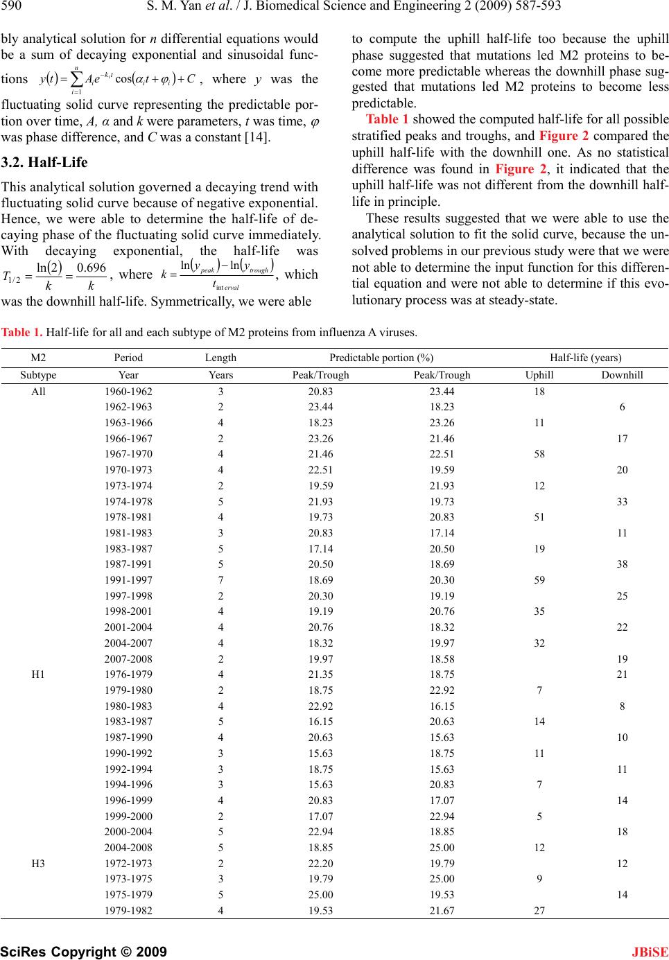 590 S. M. Yan et al. / J. Biomedical Science and Engineering 2 (2009) 587-593 SciRes Copyright © 2009 ly analyticerential equations would ating solid curve representin olution governed a decaying trend with al solution for n diffb be a sum of decaying exponential and sinusoidal func- tions CteAty n tk i i cos , where y was the fluctug the predictable por- tion over time, A, α and k were parameters, t was time, was phase difference, and C was a constant [14]. 3.2. Half-Life i ii 1 JBiSE This analytical s fluctuating solid curve because of negative exponential. Hence, we were able to determine the half-life of de- caying phase of the fluctuating solid curve immediately. With decaying exponential, the half-life was k k T696.02ln 2/1 , where erval troughpeak yy klnln , which alf-life. Sre able tint was the downhill hymmetrically, we we to compute the uphill half-life too because the uphill owed the computed half-life for all possible st uggested that we were able to use the an able 1. Half-life for all and each subtype of M2 proteins from influenza A viruses. ) Half-life (years) phase suggested that mutations led M2 proteins to be- come more predictable whereas the downhill phase sug- gested that mutations led M2 proteins to become less predictable. Table 1 sh ratified peaks and troughs, and Figure 2 compared the uphill half-life with the downhill one. As no statistical difference was found in Figure 2, it indicated that the uphill half-life was not different from the downhill half- life in principle. These results s alytical solution to fit the solid curve, because the un- solved problems in our previous study were that we were not able to determine the input function for this differen- tial equation and were not able to determine if this evo- lutionary process was at steady-state. T M2 Period Length Predictable portion (% Se Peak/TrTrough Uphihill ubtypYear Years ough Peak/ll Down All 192 60-1963 20.83 23.44 18 1962-1963 2 23.44 18.23 6 1963-1966 4 18.23 23.26 1 17 58 20 12 33 51 19 38 59 25 35 22 32 1 H 14 1 1 1 18 12 H 12 14 1979-1982 4 19.53 21.67 27 1 1966-1967 2 23.26 21.46 1967-1970 4 21.46 22.51 1970-1973 4 22.51 19.59 1973-1974 2 19.59 21.93 1974-1978 5 21.93 19.73 1978-1981 4 19.73 20.83 1981-1983 3 20.83 17.14 11 1983-1987 5 17.14 20.50 1987-1991 5 20.50 18.69 1991-1997 7 18.69 20.30 1997-1998 2 20.30 19.19 1998-2001 4 19.19 20.76 2001-2004 4 20.76 18.32 2004-2007 4 18.32 19.97 2007-2008 2 19.97 18.58 9 1 1976-1979 4 21.35 18.75 21 1979-1980 2 18.75 22.92 7 1980-1983 4 22.92 16.15 8 1983-1987 5 16.15 20.63 1987-1990 4 20.63 15.63 0 1990-1992 3 15.63 18.75 1 1992-1994 3 18.75 15.63 11 1994-1996 3 15.63 20.83 7 1996-1999 4 20.83 17.07 4 1999-2000 2 17.07 22.94 5 2000-2004 5 22.94 18.85 2004-2008 5 18.85 25.00 3 1972-1973 2 22.20 19.79 1973-1975 3 19.79 25.00 9 1975-1979 5 25.00 19.53 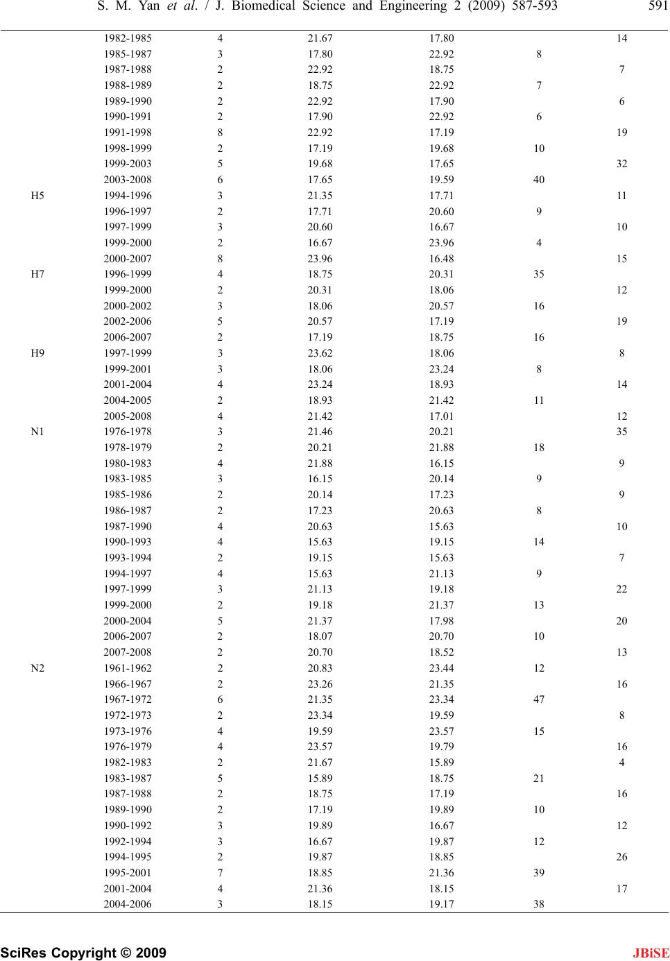 S. M. Yan et al. / J. Biomedical Science and Engineering 2 (2009) 587-593 591 SciRes Copyright © 2009 JBiSE 1982-1985 4 21.67 17.80 14 1985-1987 3 17.80 22.92 8 1987-1988 2 22.92 18.75 7 1988-1989 2 18.75 22.92 7 1989-1990 2 22.92 17.90 6 1990-1991 2 17.90 22.92 6 1991-1998 8 22.92 17.19 19 1998-1999 2 17.19 19.68 10 1999-2003 5 19.68 17.65 32 2003-2008 6 17.65 19.59 40 H H H N 35 18 N 21 5 1994-1996 3 21.35 17.71 11 1996-1997 2 17.71 20.60 9 1997-1999 3 20.60 16.67 10 1999-2000 2 16.67 23.96 4 2000-2007 8 23.96 16.48 15 7 1996-1999 4 18.75 20.31 35 1999-2000 2 20.31 18.06 12 2000-2002 3 18.06 20.57 16 2002-2006 5 20.57 17.19 19 2006-2007 2 17.19 18.75 16 9 1997-1999 3 23.62 18.06 8 1999-2001 3 18.06 23.24 8 2001-2004 4 23.24 18.93 14 2004-2005 2 18.93 21.42 11 2005-2008 4 21.42 17.01 12 1 1976-1978 3 21.46 20.21 1978-1979 2 20.21 21.88 1980-1983 4 21.88 16.15 9 1983-1985 3 16.15 20.14 9 1985-1986 2 20.14 17.23 9 1986-1987 2 17.23 20.63 8 1987-1990 4 20.63 15.63 10 1990-1993 4 15.63 19.15 14 1993-1994 2 19.15 15.63 7 1994-1997 4 15.63 21.13 9 1997-1999 3 21.13 19.18 22 1999-2000 2 19.18 21.37 13 2000-2004 5 21.37 17.98 20 2006-2007 2 18.07 20.70 10 2007-2008 2 20.70 18.52 13 2 1961-1962 2 20.83 23.44 12 1966-1967 2 23.26 21.35 16 1967-1972 6 21.35 23.34 47 1972-1973 2 23.34 19.59 8 1973-1976 4 19.59 23.57 15 1976-1979 4 23.57 19.79 16 1982-1983 2 21.67 15.89 4 1983-1987 5 15.89 18.75 1987-1988 2 18.75 17.19 16 1989-1990 2 17.19 19.89 10 1990-1992 3 19.89 16.67 12 1992-1994 3 16.67 19.87 12 1994-1995 2 19.87 18.85 26 1995-2001 7 18.85 21.36 39 2001-2004 4 21.36 18.15 17 2004-2006 3 18.15 19.17 38 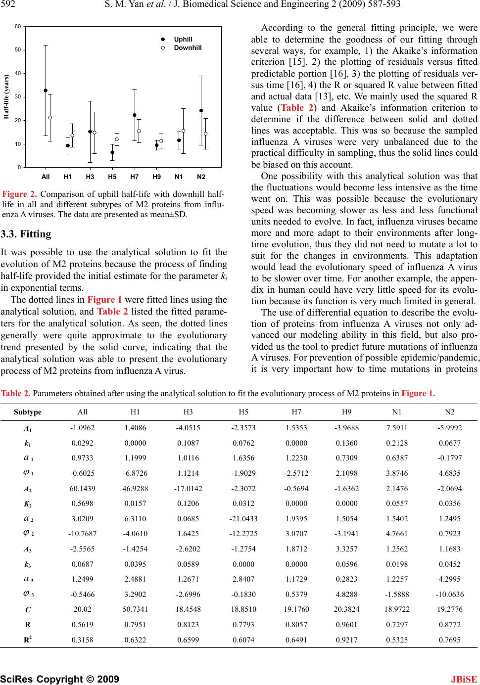 592 S. M. Yan et al. / J. Biomedical Science and Engineering 2 (2009) 587-593 SciRes Copyright © 2009 AllH1H3H5H7H9N1N2 Half-life (years) 0 10 20 30 40 50 60 Uphill Downhill Figure 2. Comparison of uphill half-life with downhill half- life in all and different subtypes of M2 proteins from influ- enza A viruses. The data are presented as mean±SD. e 2 proteins because the process of finding Accordingeneral fitting principle, were able to deterthe goodnes our fittingrough se fit Subtype All H1 H3 H5 H7 H9 N1 N2 to the g we mine s of th veral ways, for example, 1) the Akaike’s information criterion [15], 2) the plotting of residuals versus fitted predictable portion [16], 3) the plotting of residuals ver- sus time [16], 4) the R or squared R value between fitted and actual data [13], etc. We mainly used the squared R value (Table 2) and Akaike’s information criterion to determine if the difference between solid and dotted lines was acceptable. This was so because the sampled influenza A viruses were very unbalanced due to the practical difficulty in sampling, thus the solid lines could be biased on this account. One possibility with this analytical solution was that the fluctuations would become less intensive as the time went on. This was possible because the evolutionary speed was becoming slower as less and less functional units needed to evolve. In fact, influenza viruses became more and more adapt to their environments after long- time evolution, thus they did not need to mutate a lot to suit for the changes in environments. This adaptation would lead the evolutionary speed of influenza A virus to be slower over time. For another example, the appen- dix in human could have very little speed for its evolu- tion because its function is very much limited in general. The use of differential equation to describe the evolu- tion of proteins from influenza A viruses not only ad- va 3.3. Fitting t was possible to use the analytical solution to fit thI evolution of M half-life provided the initial estimate for the parameter ki in exponential terms. The dotted lines in Figure 1 were fitted lines using the analytical solution, and Table 2 listed the fitted parame- ters for the analytical solution. As seen, the dotted lines generally were quite approximate to the evolutionary trend presented by the solid curve, indicating that the analytical solution was able to present the evolutionary process of M2 proteins from influenza A virus. Table 2. Parameters obtained after using the analytical solution to nced our modeling ability in this field, but also pro- vided us the tool to predict future mutations of influenza A viruses. For prevention of possible epidemic/pandemic, it is very important how to time mutations in proteins the evolutionary process of M2 proteins in Figure 1. A1 -1.0962 1.4086 -4.0515 -2.3573 1.5353 -3.9688 7.5911 -5.9992 k1 0. 0 0 0. 0 0. 0. 0. 0292.0000.10870762.0000136021280677 a1 0.9733 1.1999 1.0116 1.6356 1.2230 0.7309 0.6387 -0.1797 1 -0.6025 -6.8726 1.1214 -1.9029 -2.5712 2.1098 3.8746 4.6835 A- K 2 60.1439 46.9288 17.0142 -2.3072 -0.5694 -1.6362 2.1476 -2.0694 2 0.5698 0.0157 0.1206 0.0312 0.0000 0.0000 0.0557 0.0356 a2 3.0209 6.3110 0.0685 -21.0433 1.9395 1.5054 1.5402 1.2495 2 -10.7687 -4.0610 1.6425 - A k 12.2725 3.0707 -3.1941 4.7661 0.7923 3 -2.5565 -1.4254 -2.6202 -1.2754 1.8712 3.3257 1.2562 1.1683 3 0.0687 0.0395 0.0589 0.0000 0.0000 0.0596 0.0198 0.0452 a3 1.2499 2.4881 1.2671 2.8407 1.1729 0.2823 1.2257 4.2995 3 -0.5466 3.2902 -2.6996 -0.1830 0.5379 4.8288 -1.5888 -10.0636 C R 20.02 50.7341 18.4548 18.8510 19.1760 20.3824 18.9722 19.2776 0.5619 0.7951 0.8123 0.7793 0.8057 0.9601 0.7297 0.8772 R2 0.3158 0.6322 0.6599 0.6074 0.6491 0.9217 0.5325 0.7695 JBiSE  S. M. Yan et al. / J. Biomedical Science and Engineering 2 (2009) 587-593 593 SciRes Copyright © 2009 from iuenza As. In tt we e fast Fourier transformis jo17-20]near ture we are abhe an Sciences (0701 and nd G. Wu. (2009) Describing evolution of he- magglutinins from influenza A viruses using a diff in Pept. Lett., 16, 794–804. n. (2002) Randomness in the primar maggluti- of influenza A virus pro- 5. nel, iviral J. Neyts. (2007) Avian influenza Developing new antiviral agents for infleatme doesre hol In- fect 48, S3–S13. 1] M.ert, Milette, s and . (2009) Universal M2 ectodomain-based influenza A vac- JBiSE nfl virusehe pasused th to do th le to use t b [3,5, alytical so . In the lution with fu fitted parameters to time the mutations. 4. ACKNOWLEDGEMENTS This study was partly supported by Guangxi Science Foundation (0907016 and 0991080) and Guangxi Academy of 09YJ17SW07). REFERENCES [1] S. Yan a eren- tial equation, Prote [2] G. Wu and S. Yay structure of protein: Methods and implications, Mol. Biol. Today, 3, 55–69. [3] G. Wu and S. Yan. (2006) Mutation trend of he nin of influenza A virus: A review from computational mutation viewpoint, Acta Pharmacol. Sin., 27, 513–526. [4] G. Wu and S. Yan. (2006) Fate teins, Protein Pept. Lett., 13, 377–384. [5] G. Wu and S. Yan. (2008) Lecture notes on computational mutation, Nova Science Publishers, New York. [6] T. Betakova. (2007) M2 protein-a proton channel of in- fluenza A virus, Curr. Pharm. Des., 13, 3231–323 [7] L. H. Pinto and R. A. Lamb. (2007) Controlling influenza virus replication by inhibiting its proton chanMol. Biosyst., 3, 18–23 [8] J. Beigel and M. Bray. (2008) Current and future ant therapy of severe seasonal and avian influenza, Antiviral Res., 78, 91–102. [9] E. De Clercq and A (H5N1) infection: Targets and strategies for chemothera- peutic intervention, Trends Pharmacol. Sci., 28, 280–285. [10] F. Hayden. (2009) uenza trnt: What the futud? Clin. . Dis., Schotsa[1 . De FW. FierX. Saelens cines: Preclinical and clinical developments, Expert Rev. Vaccines, 8, 499–508. [12] Influenza virus resources, (2009) http://www.ncbi.nlm.nih.gov/genomes/FLU/Database/mu ltiple.cgi. [13] SPSS Inc., (2002) Sigm [14] aPlot for Windows, Version 8.02. Bayesian and nonlinear hys. Res. Commun., 333, 70–78. G. Wu. (1996) Fit fluctuating blood drug concentration: A beginner’s first note, Pharmacol. Res., 33, 379–383. [15] K. Yamaoka, T. Nakagawa and T. Uno. (1978) Applica- tion of Akaike’s information criterion (AIC) in the eva- luation of linear pharmacoketic equations, J. Pharma- cokinet. Biopharm., 6, 165–175. [16] G. Wu, P. Cossettini and M. Furlanut. (1996) Prediction of blood cyclosporine concentrations in haematological patients with multidrug resistance by one-, two- and three-compartment models using least squares methods, Pharmacol. Res., 34, 47–57. [17] G. Wu and S. Yan. (2006) Timing of mutation in hemag- glutinins from influenza A virus by means of amino-acid distribution rank and fast Fourier transform, Protein Pept. Lett., 13, 143–148. [18] G. Wu and S. Yan. (2005) Timing of mutation in hemag- glutinins from influenza A virus by means of unpredict- able portion of amino-acid pair and fast Fourier trans- form, Biochem. Biop [19] G. Wu and S. Yan. (2005) Searching of main cause lead- ing to severe influenza A virus mutations and conse- quently to influenza pandemics/epidemics, Am. J. Infect. Dis., 1, 116–123. [20] S. Yan and G. Wu. (2009) Prediction of mutation position, mutated amino acid and timing in hemagglutinins from North America H1 influenza A virus, J. Biomed. Sci. Eng, 2, 190–199. |

