Energy and Power Engineering, 2009, 94-99
doi:10.4236/epe.2009.12015 Published Online November 2009 (http://www.scirp.org/journal/epe)
A New Multi-Method Combination Forecasting
Model for ESDD Predicting
Haiyan SHUAI, Qingwu GONG
1School of Electrical Engineering, Wuhan Technical College of Communications,
Wuhan University, Wuhan, China
2School of Electrical Engineering, Wuhan University, Wuhan, China
Abstract: Equal Salt Deposit Density (ESDD) is a main factor to classify contamination severity and draw
pollution distribution map. The precise ESDD forecasting plays an important role in the safety, economy and
reliability of power system. To cope with the problems existing in the ESDD predicting by multivariate linear
regression (MLR), back propagation (BP) neural network and least squares support vector machines
(LSSVM), a nonlinear combination forecasting model based on wavelet neural network (WNN) for ESDD is
proposed. The model is a WNN with three layers, whose input layer has three neurons and output layer has
one neuron, namely, regarding the ESDD forecasting results of MLR, BP and LSSVM as the inputs of the
model and the observed value as the output. In the interest of better reflection of the influence of each single
forecasting model on ESDD and increase of the accuracy of ESDD prediction, Morlet wavelet is used to con-
struct WNN, error backpropagation algorithm is adopted to train the network and genetic algorithm is used to
determine the initials of the parameters. Simulation results show that the accuracy of the proposed combina-
tion ESDD forecasting model is higher than that of any single model and that of traditional linear combina-
tion forecasting (LCF) model. The model provides a new feasible way to increase the accuracy of pollution
distribution map of power network.
Keywords: equal salt deposit density, multivariate linear regression, BP neural network, least squares support
vector machines, combination forecasting, wavelet neural network
1. Introduction
Exposed to dirty environment, surfaces of insulators will
be polluted. After being wetted, the polluted layers will
deduce insulators’ insulation capability which often in-
vites pollution flashover. According to the operation ex-
periences of power sectors, pollution flashover is one of
the main factors causing power accidents. In recent years
[1,2], there have happened several large area pollution
flashovers in some locals or the whole country, which
resulted in large area power blackout. Among all the
causes resulting in pollution flashover, the lag and the
inaccuracy of pollution distribution map of power net-
work is a primary one. Equal Salt Deposit Density
(ESDD) is the equivalent amount of NaCl that would
yield the same conductivity at complete dilution [3],
which is the dominant factor to classify contamination
severity and draw pollution distribution map. At present,
the methods of ESDD forecasting are mainly traditional
multivariate linear regression (MLR) technique [4,5],
back propagation (BP) neural network [6,7], and least
squares support vector machines (LSSVM) [8,9]. Com-
bination forecasting integrates the useful information of
all single forecasting models and generally considers
each forecasting result; hence it can more systemically
and comprehensively reflect the changes of an object
than a single model does. J. M. Bates and C. J. W.
Granger proved the combination of two or more than two
agonic single forecasting models can produce the result
better than that of each single model, which showed
combination forecasting method can increase prediction
accuracy [10].
To improve ESDD forecasting accuracy, a nonlinear
combination forecasting model based on wavelet neural
network (WNN) for ESDD is proposed. The model is a
WNN with three layers, whose inputs are the forecasting
results of the three ESDD forecasting models mentioned
above, i.e., MLR, BP and LSSVM, and outputs are the
observed values of ESDD. For the sake of better reflec-
tion of the influence of each single forecasting model on
ESDD and increase of the accuracy of ESDD prediction,
Morlet wavelet is used to construct WNN and error
backpropagation algorithm is adopted to train the net-
work. Simulation results show that the accuracy of the
proposed combination ESDD forecasting model is higher
than that of any single model and also higher than that of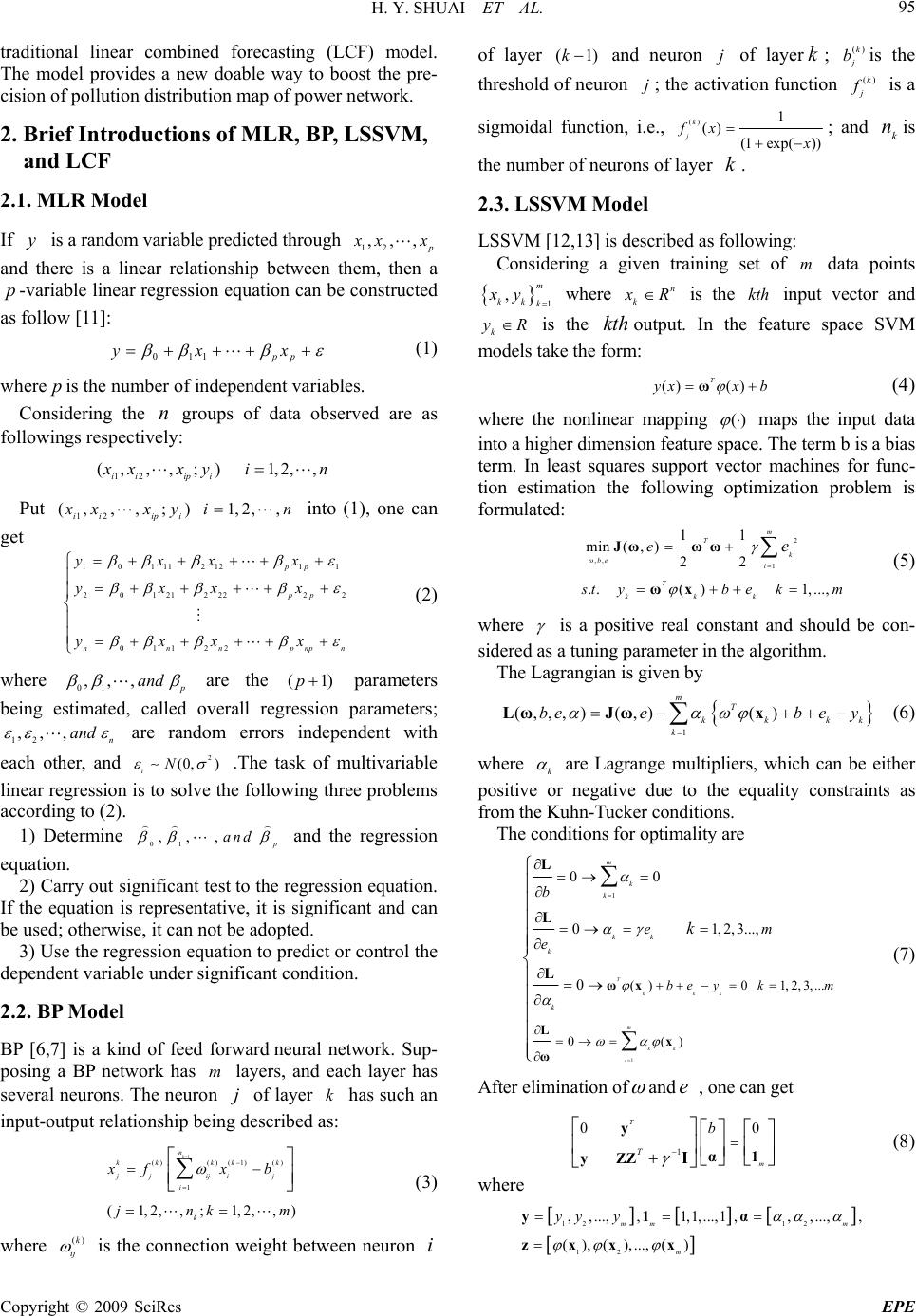

H. Y. SHUAI ET AL. 95
traditional linear combined forecasting (LCF) model.
The model provides a new doable way to boost the pre-
cision of pollution distribution map of power network.
2. Brief Introductions of MLR, BP, LSSVM,
and LCF
2.1. MLR Model
If is a random variable predicted through y12 ,,,
p
x
xx
and there is a linear relationship between them, then a
-variable linear regression equation can be constructed
as follow [11]:
p
011 pp
yx x

   
(1)
where is the number of independent variables. p
Considering the groups of data observed are as
followings respectively:
n
12
(,,, ;)1,2,,
ii ipi
x
xxyin
Put 12 (,,, ;)1,2,,
ii ipi
x
xxyi n
n
into (1), one can
get
101112121 1
201212222 2
01122
pp
pp
nnnpnp
yxx x
yxxx
yxx x
 

 

 

 
 

 











(2)
where 01
,,,
p
and

 
,n and
are the parameters
being estimated, called overall regression parameters;
(1)p
12
,,

 
(0,
iN
 are random errors independent with
each other, and 2)

  .The task of multivariable
linear regression is to solve the following three problems
according to (2).
1) Determine 01
,,,
p
and

  




m


and the regression
equation.
2) Carry out significant test to the regression equation.
If the equation is representative, it is significant and can
be used; otherwise, it can not be adopted.
3) Use the regression equation to predict or control the
dependent variable under significant condition.
2.2. BP Model
BP [6,7] is a kind of feed forward neural network. Sup-
posing a BP network has layers, and each layer has
several neurons. The neuron of layer has such an
input-output relationship being described as:
m
jk
1
()() ( 1)()
1
1, 2,,1, 2,,
k
n
kkkk k
jjijij
i
k
xfx b
jnk





 





(3)
where ()k
ij

is the connection weight between neuron
of layer
i
(1)k

and neuron
j
of layer; is the
threshold of neuron
k()k
j
b
j
; the activation function )(k
j
f
is a
sigmoidal function, i.e., () 1
()fx
(1 exp(
k
j))
x

k

; and is
the number of neurons of layer .
k
n
2.3. LSSVM Model
LSSVM [12,13] is described as following:
Considering a given training set of m data points
 
,m
kk
k
xy 1

where n
k
x
R is the input vector and kth
k
yR

is the output. In the feature space SVM
models take the form:
kth
()yx b()x
T


ω (4)
where the nonlinear mapping ()

 maps the input data
into a higher dimension feature space. The term b is a bias
term. In least squares support vector machines for func-
tion estimation the following optimization problem is
formulated:
2
,,
min
. .
be 1
(
( )
m
T
k
i
T
kkk
11
22
, )e
1,...,
s
ty ek
e 


b m



 
 Jωω
x
ω
ω
(5)
where

is a positive real constant and should be con-
sidered as a tuning parameter in the algorithm.
The Lagrangian is given by

k
y

T
1
(,(( )
m
kk
k


,, )be ,)e k b e  


LωJωx (6)
where k

are Lagrange multipliers, which can be either
positive or negative due to the equality constraints as
from the Kuhn-Tucker conditions.
The conditions for optimality are
1
()
0(
00
kk




x
1
0 1,
..,
T
kk
m
kk
i
m
k
be k
b
em
e
k





 
 





















ω
L
x
ω
L
2,3,...
)
1, 2,
y

0
0
k
k
k





L
L
3.
k


m
(7)
After elimination of

and , one can get e
1
0
T
m








y
1
yZ I
0
T
Z
b



α
(8)
where







1
12
1,1,. ,
),()
m
y 


x
12
, ,...,
(), (
yy
 zx
2
,...,,
...,
mm
y1
x
..,1, α,
m


H. Y. SHUAI ET AL.
96
From application of the Mercer condition one can ob-
tain (,)()(),,1, 2,...,
T
iji j
K
ij m   Ωxxx x. This finally
results into the following LS-SVM model for function
estimation
1
(, )
m
kk
k
yK 


xx b
(9)
2.4. LCF Model
Linear combination forecasting model [14] takes the
form:
112233
123
1(0,1, 2, 3)
tttt
i
gkgkg kg
kkkk i
 
  


 (10)
where t
g
is the value of the linear combination fore-
casting model; 1t
g
, 2t
g
and 3t
g
are the forecasting
values of the single forecasting models respectively,
namely, MLR, BP and LSSVM; and , and are
the weighted coefficients of the three single models re-
spectively. To the linear combination forecasting method,
its main task is to adopt optimization measures to obtain
the optimal weighted coefficients which can make the
error sum of squares of the combined forecasting be
least.
1
k2 k3 k
3. WNN Combination Forecasting Model for
ESDD Predicting
Supposing , and are the ESDD pre-
dicting values of MLR, BP and LSSVM respectively,
is the measured value. One can use , and
to construct a nonlinear combination function [15]
1i
z2i z3i zith
i
h
ith 1i z2i z
3i
z
123
()( ,,)
ii iiii
hZ zzz 
  (11)
where,

is the nonlinear function and is the com-
bined forecasting value. In this paper, WNN is used to
design the nonlinear function
i
h


.
It is known the nature of wavelet transform [16] is an
integral transform between different parameters.
 ,()(,,)
ab
wab fxgabxdt


 
 (12)
where, 1
(,,)( )
||
x
b
gabxg a
a

 is called wavelet basis
and ()
g
x
,)
called mother wavelet. and are
termed as scaling factor and translation factor of
ab
(,
g
abx respectively. To


f
x, the resolution of its
local structure can be realized through adjusting 、,
namely, gearing the scale and position of wavelet basis
window.
ab
WNN [17] is a model which, based upon wavelet
analysis, possesses neural network thread. In other words,
WNN adopts nonlinear wavelet basis to replace com-
mon-used Sigmoid function in traditional neural network.
Through linear superposition of nonlinear wavelet basis
selected, the combination of the ESDD data of all single
forecasting models is realized. The nonlinear combina-
tion function in (11) can be fitted as follow, by adopting
wavelet basis (,,)
g
abx :
1
1
ˆ() ()
L
ji jk k
mj
ii k
kk
vz b
hZ ga 







(13)
where ()
i
Z

3L
is the ESDD value of nonlinear combina-
tion forecasting corresponding to the measured one ;
expresses the prediction value of the
model,
i
h
jth
ji
zith

; 123 , )
iii
(,
Z
zzz; k

、 、 、 are
the weighted coefficient between output terminal and the
hidden layer node, the weighted between the
input and the hidden layer node, the translation
factor and scaling factor of the wavelet basis re-
spectively; the number of wavelet basis is 7, ac-
cording to the empirical formula . Considering
Morlet wavelet possessing relatively good localization
and smoothness, it will be selected in (13).
jk
v
2n
k
b
m
k
a
kth jth
kth
kth
1
2
()cos(1.75)exp()
2
x
gx x


i
(14)
Figure 1 shows the structure of WNN. There are
input nodes- and one output node-
3
123
,,
ii
zz z()
i
Z

.
The objective of using WNN to carry out regression
analysis is to determine the network parameters-k

、
、 and by which
jk
vk bk a()
i
Z

can be fitted optimally
with .
i
hk

、 、 and can be optimized via
Minimum Mean Square Error (MMSE) energy function
as follow.
jk
vk
bk a
12
11
1[( ))
2
L
jk jik
Im j
k
ik k
vzb
Eg
a




]
i
h



 
(15)
Figure1. The structure of WNN

H. Y. SHUAI ET AL. 97
where,
I
is the number of training samples and is
the observed value.
i
h
ith
To gain the optimal k

、 、 and is to
minimize (15). In this article, gradient descent algorithm
is used as WNN learning principle. The details are as
followings:
jk
vk bk a
1) Set the objective error function value;
2) Initialize k

、 、 and between [1
jk
vk bk a,1]

by using Genetic Algorithm [18];
3) Select randomly a training mode, and input the
learning samples and corresponding output ;
ji
zi h
4) Work out the predicting value of the network ,
the followings are the details:
ˆ
i
h
a) Calculate the gradient of each parameter;
Let ，
*
1
L
jk ji
j
zv

z
*
k
k
zb
Sa

， then the gradients of
(15) are respectively:
1
*
[()][]
I
ii
i
k
k
k
EZhg
zb
a



 



2
1
2
2
1
2
1
[()][cos(1.75) exp()
2
1
1.75 sin(1.75) exp()]
2
[()][cos(1.75) exp()
2
1
1.75 sin(1.75) exp()]
2
[()]
I
iik
i
j
k k
ji
k
I
iik
i
jk k
k
I
iik
i
k
E
Zh S
v
S
Sz
a
E
ZhS
b
S
S
a
EZh
a






 

 
 

 
 




SS
a
SS
a
2
2
2
[cos(1.75) exp()
2
1.75 sin(1.75) exp()]
2
k
k
SS
S
a
SS
S
a

 
b) Introduce momentum factor

to amend each pa-
rameter;
(1) ()()
(1) ()()
(1)()()
(1)()()
kk k
k
jk jkjk
jk
kk k
k
kk k
k
E
tt t
E
vt vtvt
v
E
bt btbt
b
E
at atat
a






 


 


 


 





where,

is the learning ratio and

is the momen-
tum factor.
c) Compute current output of WNN: put current pa-
rameters into (13) to get current output of the network;
d) Numerate error function value. When the error is
less than the set one, the learning process is terminated;
otherwise, turns to step (3).
4. Appraisal of Forecasting
In order to evaluate the prediction effects of the combi-
nation model comprehensively, according to the practice
and principle, the paper uses relative error

and aver-
age relative error

to evaluate the accuracy of the
prediction.
100%
ˆ
i
ii
y
yy
 
 (16)
1i
100%
ˆ
1
y
I
ii
i
yy
I




 (17)
where are the observed values and are the pre-
dicted ones. These values reflect comprehensively the
prediction results. The smaller
i
yˆi y

and

are, the better
the generalization of the model and the corresponding
parameters are.
5. Experimental Results
On the basis of the model principles and modeling steps
in the text, Matlab 7.0 is adopted to write the ESDD pre-
diction programs based on WNN. References [4–7,9]
show there is a close relationship between insulators
ESDD and meteorological factors. So, for each single
model, 120 samples of the historical meteorological data
and ESDD data provided by “Optical Sensor System for
the ESDD Monitoring of Transmission Equipment” (de-
veloped by Wuhan High Voltage Research Institute and
Wuhan Kangpu Changqing Software Company) installed
on the ESDD monitoring spot of Qingshan District, Wu-
han ,from April to June in 2006, are regarded as training
set and forecasting set, where 90 samples belong to
training set, and the rest 30 samples to test set. Table 1
shows the comparisons between WNN combination
forecasting model and LCF, MLR, BP and LSSVM.
Figure 2. Optical sensor system for the ESDD monitoring of
transmission equipment

H. Y. SHUAI ET AL.
98
Table 1. Comparison of forecasting results of ten ESDD
Combination forecasting Single forecasting
WNN LCF MLR BP LSSVM
Times Actual
（mg/cm2） Forecasting
（mg/cm2） (%)

Forecasting
（mg/cm2）(%)

Forecasting
（mg/cm2）(%)

Forecasting
（mg/cm2）(%)

Forecasting
（mg/cm2） (%)

2006.4.8 0.0268 0.0278 3.73 0.0252 5.970.0286 6.720.0249 7.09 0.0284 5.97
2006.4.16 0.0263 0.0271 3.04 0.0276 4.940.0291 10.650.0247 6.08 0.0286 8.75
2006.4.21 0.0390 0.0381 2.31 0.0375 3.850.0412 5.640.0421 7.95 0.0363 6.92
2006.5.3 0.0353 0.0362 2.55 0.0367 3.970.0331 6.230.0334 5.38 0.0342 3.12
2006.5.8 0.0232 0.0244 5.17 0.0244 3.610.0248 6.450.0251 8.19 0.0247 6.47
2006.5.13 0.0264 0.0255 3.41 0.0251 4.920.0239 9.470.0292 10.61 0.0244 7.58
2006.5.21 0.0487 0.0497 2.05 0.0517 6.160.0534 9.650.0527 8.21 0.0460 5.54
2006.6.1 0.0432 0.0414 4.17 0.0421 2.550.0463 7.170.0410 5.09 0.0455 5.32
2006.6.9 0.0459 0.0442 3.70 0.0481 4.790.0491 6.970.0427 6.97 0.0482 5.01
2006.6.18 0.0467 0.0484 3.64 0.0491 5.140.0411 11.990.0488 4.50 0.0451 3.43
(%) 
3.377 4.590 8.094 7.007 5.811
Figure 3. Comparison between the predicted and the measured
compared with linear combination model, WNN combi-
nation model presented in the paper is more stable and
practical, and can improve efficiently forecasting preci-
sion. Using the ESDD predicted by WNN combination
forecasting model to divide pollution area can effectively
increase the accuracy of pollution distribution map.
From Table 1, it can be seen that the average relative
error of MLR is 8.09 which is the biggest one
among those of the five forecasting models, and that of
WNN is , the least one , and each relative error
of WNN is less than . The average relative error of
LCF is which is only bigger than that of WNN.
Besides, the maximum relative error of LCF, MLR, BP
and LSSVM are 6.16 , , and
respectively; while that of WNN is only .
This indicates that the prediction accuracy of combina-
tion model is higher than that of each single model, and
4%
6%
%
3.377%
4.590%
11.99% 10.61%
5.17.58% 7%
6. Conclusions
ESDD is a main factor to classify contamination severity
and draw pollution areas map of power network, hence its
accuracy directly influences the precision of pollution

H. Y. SHUAI ET AL. 99
distribution map, and further affects the insulation capa-
bility of power system.
The WNN combination forecasting model combined
with multivariable linear regression technique, BP neural
network and least squares support vector machines avoids
the limitations of linear combination model and single
forecasting model, so it can boost the forecasting accu-
racy, especially deduce maximum relative error, in other
words, it can decline predicting risk. The simulation re-
sults in Table 1 show in the five models, the prediction
accuracy of WNN combination model is the highest one,
namely, the values of WNN are closest to the observed
ones. The ESDD values produced by WNN combination
forecasting model can better meet the request of drawing
pollution distribution map of power network. The model
proposed by the paper is an effective and doable way for
ESDD forecasting and provides a new thinking for the
computerization of drawing pollution distribution map.
REFERENCES
[1] Y. Hu, “The analysis of ‘2.22 pollution flashover of net-
work’ and measure for anti-pollution flashover,” High
Voltage Engineering, Vol. 27, pp. 30–32, April 2001.
[2] Y. Liu and J. K. Wang, “Analysis of large area pollution
flashover occurred in Shaanxi power network on Dec.18,
2000 and preventative measures for similar accidents,”
Power System Technology, Vol. 26, pp. 82–85, June
2002.
[3] Pollution Classification and External Insulation Selection
for Electrical Power System, State Grid Standard Q/
GDW152-2006, December 2006.
[4] A. S. Almad, H. Ahmad, M. A. Salam, and Saad Ahmad,
“Regression technique for prediction of salt contamina-
tion severity on high voltage insulators,” in Annual Re-
port Conference on Electrical Insulation and Dielectric
Phenomena, pp. 218–221, 2000.
[5] A. S. Almad, H. Ahmad, M. A. Salam, T. Tamsir, Z. Bun-
tat, and M. W. Mustafa, “Prediction of salt contamination
on high voltage insulators in rainy season using regres-
sion technique,” Proceedings of TENCON, Vol. 3, pp.
184–189, 2000.
[6] M. A. Salam, S. M. Ai-Alawi, and A. A Maqrashi, “Pre-
diction of equivalent deposit density of contaminated
glass plates using artificial neural networks,” Journal of
Electrostatics, Vol. 66, pp. 526–530, May 2008.
[7] A. S. Almad, P. S. Ghosh, H. Ahmad, and S. A .K. Aljunid,
“Assessment of ESDD on high-voltage insulators using
artificial neural network,” Electric Power System Re-
search, Vol. 72, pp. 131–136, December 2004.
[8] S. B. Jiao, D. Liu, G. Zheng, and Q. Zhang, “Forecasting
the ESDD of insulator based on least squares support
vector machine,” Proceedings of the CSEE, Vol. 26, pp.
149–153, January 2006.
[9] F. H. Shu and W. X. Zhang, “A prediction model for in-
sulator’s ESDD based on least square support vector ma-
chine,” High Voltage Apparatus, Vol. 44, pp. 420–423,
October 2008.
[10] J. M. Bate and C. W. J. Granger, “The combination of
forecastings,” Operational Research Quarterly, Vol. 20,
pp. 451–468, 1969.
[11] Y. Liu. “Mathematical model of multivariable linear re-
gression,” Journal of Shenyang Institute of Engineering,
Vol. 1, pp. 128–129, Junuary 2005.
[12] J. A. K. Suykens and J. Vandewalle. “Least squares sup-
port vector machine classifiers,” Neural Process Letters,
Vol. 9, pp. 293–300, 1999.
[13] J. A. K. Suykens, L. Lukas, P. Van Dooren, B. Demoor,
and J. Vandewalle, “Least squares support vector machine
classifiers: A large scale algorithm,” ECCTD’99 Euro-
pean Conference on Circuit Theory and Design, pp.
293–300, 1999.
[14] Y. K. Ma and X. W. Tang, “Research on the problem of
optimizing linear combination forecasting model,” Sys-
tem Engineering – Theory & Practice, Vol. 9, pp. 110–
123, September 1998.
[15] X. H. Wen and M. J. Niu, “A new nonlinear combined
forecasting method on the basis of neural networks,” Sys-
tem Engineering-Theory & Practice, Vol. 12, pp. 66–72,
December 1994.
[16] S. X. Li, “Wavelet transform and its applications,” Higher
Education Press, Beijing, pp. 11–15, 1997.
[17] Q. X. Cuo and L. Liu, “Driving force prediction for in-
clusion complexation of 2-cyclodextrim with benzene de-
rivatives by a wavelet neural network,” Chemical Physics
Letters, Vol. 290, pp. 514–518, 1998.
[18] H. F. Liang, G. Y. Tu, and H. W. Tang, “Application of
genetic algorithm neural network for short term load fore-
casting of power system,” Power System Technology, Vol.
25, pp. 49–53, January 2001.