Journal of Environmental Protection, 2011, 2, 1317-1330
doi:10.4236/jep.2011.210152 Published Online December 2011 (http://www.SciRP.org/journal/jep)
1317
Variability in Road Runoff Pollution by Polycyclic
Aromatic Hydrocarbons (PAHs) in the Urbanized
Area Adjacent to Biscayne Bay, Florida
Diana Mitsova1, Jaap Vos1, Piero Gardinali2, Inna Stafeychuk1
1School of Urban and Regional Planning, Florida Atlantic University, Fort Lauderdale, USA; 2Department of Chemistry & Biochem-
istry and Southeast Environmental Research Center (SERC), Florida International University, North Miami, USA.
Received September 8th, 2011; revised October 14th, 2011; accepted November 17th, 2011.
ABSTRACT
Polycyclic aromatic hydrocarbons (PAHs) were consistently documented in the sediments of the canals draining into
Biscayne Bay. The study examines the contribution of urban runoff to PAHs discharges. Subtropical climatic conditions
associated with prolonged dry seasons often exacerbate the problem of PAHs pollution as the initial storms of the wet
season wash off pollutants accumulated over time. Road runoff samples were collected at two sites with different levels
of traffic at the end and at the beginning of the wet season. Storm-event mass first flush was found to occur inconsis-
tently. Higher levels of PAH pollution were found at both sites after an extended dry season. The Kendall’s tau test used
to measure the association between antecedent dry days and flow-weighted PAH concentrations were found to be sta-
tistically significant. The correlation between traffic intensity and PAHs levels in road runoff was found not to be statis-
tically significant. High-molecular-weight PAHs originating in vehicle exhaust emissions appeared to dominate PAH
concentrations in road runoff. The Friedman’s test showed overall similarity in PAHs composition profiles between
seasons with the exception of low-molecular weight PAHs.
Keywords: PAHs, Storm-Event Mass First Flush, Seasonal Variability, Annual Average Daily Traffic
1. Introduction
Polycyclic aromatic hydrocarbons (PAHs) are an assem-
bly of over 100 semi-volatile organic compounds consist-
ing of two or more fused benzene rings. They are com-
monly present in the urban environment and are often as-
sociated with a variety of diffuse natural and anthropo-
genic sources. PAHs vary in prevalence, toxicity and per-
sistence in the environment. Higher molecular weight PAHs
often associated with by-products of incomplete combus-
tion are considered persistent organic pollutants (POPs)
with relatively long half-lives in soils and sediment [1].
Awareness of the omnipresence of PAHs and their often
elevated background levels in highly urbanized areas has
prompted a number of recent studies [2-6] as well as in-
creased attention from the USEPA and the Agency for
Toxic Substances and Disease Registry (ATSDR) [7].
Pollutant discharges carried by stormwater runoff to
Biscayne National Park and Aquatic Preserve are known
to include suspended solids, nitrogen, phosphorus, cad-
mium, copper, lead, zinc, oil, grease, litter and organic
waste [8-12]. The presence of aliphatic and aromatic hy-
drocarbons in the sediments of Biscayne Bay has been
investigated since the 1980s. Corcoran et al. [9] com-
pleted The Biscayne Bay Hydrocarbon Study, a large-
scale analysis of the spatial distribution of the hydrocar-
bons in estuarine sediments. Cantillo et al. [11] contin-
ued the investigation of PAHs content in mollusks and
sediments in South Florida as part of the NOAA National
Status and Trends Program. Earlier studies consistently
documented the presence of PAHs in sediments of Mi-
ami River and the Biscayne Bay [9,11,13]. Comprehen-
sive recent studies found various levels of PAHs in sedi-
ment samples collected from the beds of the canals and
lower Miami River in Miami-Dade County [13-15]. Al-
though the extent of PAH contamination of the sediments
of Biscayne Bay is well established, the contribution of
urban runoff as a source of origin of PAHs requires fur-
ther investigation.
PAHs tend to adhere to particles and are typically found
in both dissolved and particulate phases in urban runoff.

Variability in Road Runoff Pollution by Polycyclic Aromatic Hydrocarbons (PAHs) in the Urbanized Area Adjacent 1318
to Biscayne Bay, Florida
Despite low concentrations, urban runoff could deliver
considerable amounts of oil and grease to the aquatic en-
vironment exclusive of spills [16]. Recent increases in
PAH input to aquatic sediments in urban areas were re-
lated to PAHs releases from an increasing number of mo-
bile sources [17]. Increased traffic activity was linked to
high levels of PAHs in urban stormwater [6,16,18-22].
The literature suggests that the presence of low-mo-
lecular weight (LMW) PAHs in runoff is indicative of
petrogenic source of origin (i.e., crankcase oil drips,
spills, etc.), while the presence of high-molecular weight
(HMW) PAHs is associated with potential pyrolytic sour-
ces (i.e., vehicle exhaust emissions, burning of organic
matter, etc.) [5,6,16,18]. Several recent studies have given
priority to pyrolytic over petrogenic sources [5,6,20]. Stein
et al. [5] found that pyrolytic sources dominate urban run-
off over petrogenic sources in the majority of storms ir-
respective of land use. Studies also consistently docu-
mented that more than 70% of total PAHs in urban run-
off consisted of high-molecular weight PAHs suggesting
deposition associated with vehicle emissions and other
airborne inputs as dominant sources of PAHs in storm-
water and sediments [5,17,23].
Most studies agree that the main driving force contrib-
uting to PAH levels include traffic intensity [21], land
use [16,23,24] and seasonality [4]. Hoffman et al. [23]
used concentration and flow data to develop loading fac-
tors as a function of land use and average daily traffic
volume. The study found that PAHs discharge rates from
highways and industrial land use were higher than those
from residential areas. Menzie et al. [20] found that
commercial and residential land use dominate PAHs re-
leases hypothesizing that secondary sources such as spills
of oil and grease enhanced the flux from atmospheric
deposition. Stein et al. [5] found a uniform distribution of
the total PAHs flux throughout the urbanized region of
Los Angeles observing that there was no significant dif-
ference in PAHs concentrations in runoff generated from
various urban land uses.
A pollutant first flush is defined relative to the po-
llutant mass carried out by the initial fraction of the run-
off volume [2-6,25,26]. Estimation of a storm first flush
involves computing the cumulative pollutant mass dis-
charge in the initial portion of the runoff volume [2,3].
Most studies suggest that estimates of the first flush pol-
lutant emissions should be based on the initial 20% to
40% of runoff volume [26,27]. Bertrand-Krajewski et al.
[26] characterized the occurrence of a first flush as 80
percent of the pollutant mass emitted in the initial 30
percent of stormwater runoff volume. Stenstrom and
Kaynahian [2] suggested a quantitative measure based on
the mass first flush ratio (MFF). MFF allows plotting the
normalized cumulative mass discharge against the cu-
mulative runoff volume. The inflection point at which the
slope of the curve exceeds 45 percent is associated with
the occurrence of a first flush event [2,3].
Several studies found that the estimation of a first
flush may be confounded by several factors including the
size of the drainage area [28], site characteristics [4], rain-
fall patterns [6,18,23] and antecedent dry days [5,6,29].
The size of the drainage area was found to be negatively
correlated with the storm first flush. A storm first flush is
rarely reported for large watersheds [28]. Lee and Bang
[29] and Zhang et al. [6] found no significant relation-
ship between pollutant discharge and the number of an-
tecedent dry days. However, in areas where the annual
distribution of rainfall events is roughly uniform, accu-
mulation of pollutants on the ground may not be as sig-
nificant as in areas characterized by extended dry periods.
Previous studies found that climatic conditions associ-
ated with prolonged dry seasons tend to increase seasonal
discharges of pollutants to receiving waters [2,4,5]. Dur-
ing these periods without or very little precipitation
various hydrocarbon species, emitted from vehicle ex-
haust or released as a result of spillage, accumulate over
pervious and impervious surfaces [5]. Significant pollut-
ant loadings delivered to aquatic environments as a result
of the seasonal first flush may affect the productivity of
the estuarine ecosystems which harbor many fish and
shellfish species, provide spawning grounds, nurseries
and shellfish beds, and secure a vital link between pri-
mary producers and larger marine organisms [16,30].
Seasonal first flush is computed similarly to the storm
first flush when both flow and pollutant concentrations
data are available [4]. In most cases, however, these data
records are difficult to obtain on a consistent basis. Sten-
strom and Kayhanian [2] suggested using normalized
precipitation data instead of flow rate to determine sea-
sonal first flush.
The primary objective of the study was to examine the
variability in PAHs distribution in runoff from roads ad-
jacent to commercial land use. The sampling and ana-
lytical approaches were designed to address research ques-
tions related to storm-event and seasonal variability in
PAHs concentrations; existence of a mass first-flush; va-
riability in flow-weighted mean concentration, massloa-
ding rate and PAH composition profiles between storm
events and seasons; determine PAHs source of origin, and
assess the impact of average daily traffic on PAHs con-
centrations in road runoff.
2. Materials and Methods
2.1. Study Area
Biscayne Bay estuary covers approximately 430 square
miles along the lower east coast of Florida (Figure 1).
The northern portion of the Bay is designated an Aquatic

Variability in Road Runoff Pollution by Polycyclic Aromatic Hydrocarbons (PAHs) in the Urbanized Area Adjacent
to Biscayne Bay, Florida
1319
Preserve (under the Florida Aquatic Preserve Act of 1975).
Biscayne National Park encompasses the southern por-
tion of the Bay. The study area is characterized by a
warm and humid subtropical climate driven by wet and
dry seasons, convective storms and tropical cyclones [31].
The wet season extends from June through September
and the dry season from October through mid-May. The
annual average temperature is 75.9˚F. The annual pre-
cipitation is 142 cm. The wettest month is June followed
by August and September [32]. Individual years may sig-
nificantly differ from this pattern. The area is character-
ized by lowlying gently sloped topography and a com-
plex hydrology resulting from the interactions of porous
substrate geology, freshwater aquifer systems, and estua-
rine and marine environments. Biscayne Bay receives
freshwater inflows from the Everglades ecosystem through
the Biscayne Bay catchment area covering approximately
940 square miles. The area drains into the Bay through a
Figure 1. Study ar ea and sampling s ites .

Variability in Road Runoff Pollution by Polycyclic Aromatic Hydrocarbons (PAHs) in the Urbanized Area Adjacent 1320
to Biscayne Bay, Florida
system of freshwater canals. The location of Biscayne
Bay along the Miami metropolitan area with a current
population of nearly 5.5 million increases its exposure
and susceptibility to a wide variety of contaminants [12].
Population growth and continuing coastal development
have affected the water quality of Biscayne Bay and the
productivity and richness of its estuarine communities
[12].
Major transportation routes in the area include I-95,
South Dixie Highway/Federal Highway 1 (S Dixie Hwy/
US1) and the Florida Turnpike. I-95 merges into South
Dixie Highway south of Miami Downtown and conse-
quently all traffic southbound is directed towards S
Dixie/US-1 resulting in heavy traffic volumes. The road
has six lanes with major intersections every 1300 - 2000
feet. The maximum 2009 annual average daily traffic
(AADT) in the study area reached 147,000. The 2009 av-
erage AADT for Miami-Dade County was 22,500 while
the median was 30,000 [33].
In selecting the appropriate sampling locations, eleven
preliminary sites were investigated. Most areas with out-
falls had points of discharge under water due to high wa-
ter table, or under pavement and fixtures. In addition, the
South Dixie Highway sites had slab-covered trenches
completely open on the bottom, in contact with the aqui-
fer. Under these conditions, collecting samples at outfalls
could not rule out mixing urban runoff with soil and
groundwater, and therefore decision was made to collect
samples at intake chambers. Two sites were selected based
on the following criteria: 1) absence of known sources of
PAHs (e.g., gas stations, recently resurfaced parking lots,
oil storage tanks, railroads, etc.); 2) magnitude of AADT
counts; 3) homogenous land use; 4) proximity to Biscay-
ne Bay; and 5) accessibility. In 2009, Site 1 located near
the C-100 canal on S Dixie/US-1 highway (Figure 1),
had an annual average daily traffic of 69,500 vehicles per
day [33]. The site is representative of the highly urban-
ized northern part of the study area. Site 2 located near
the intersection of the 312th Street and Homestead Hos-
pital Plaza Exit of the Florida Turnpike in the City of
Homestead, Florida, had an average annual daily traffic
of 19,600 vehicles per day. The second site is representa-
tive of the less developed southern part of the study area.
Both sites are adjacent to commercial land use.
2.2. Sampling Design
The sampling procedures were in compliance with the
NDPES Storm Water Sampling Guidance [34]. The do-
cument recommends collecting oil and grease contami-
nated water in 1 L amber certified glass containers ma-
nually due to the tendency of oil and grease to adhere to
surfaces [34]. Automatic samplers were not used to avoid
transferring grab samples from one container to another.
Field collected samples were stored at 4˚C in the dark
until arrival to the laboratory. Two samples during each
storm event were collected simultaneously as part of the
quality assurance procedures.
Rainfall intensity was measured with Global Water’s
RG200 Rain Gauge (a tipping bucket). The resolution of
the tipping is 0.254 mm with accuracy of 3%. The flow
rate was estimated based on field measurements of flow
velocity. Each time when a measurement of velocity was
taken, depth and width of the flow were measured and
recorded. Archived precipitation data were collected from
weather stations located in Miami, Palmetto Bay, Cutler
Bay and Homestead.
2.3. Laboratory Analysis and Quality Assurance
Road runoff samples were analyzed by gas chromatog-
raphy-mass spectrometry (GC/MS) and fluorescence spec-
troscopy (FS). The analyses were conducted by the Envi-
ronmental Analysis Research Laboratory, Southeast Envi-
ronmental Research Center (SERC), Department of
Chemistry & Biochemistry at Florida International Uni-
versity. Water samples (1-Liter) were extracted by liq-
uid-liquid extraction against methylene chloride using a
modification of EPA 3510 as described by EARL-SOP-
2000-103.1. Sediment samples were extracted by accel-
erated solvent extraction (ASE) using modifications of
EPA method 3545. Sediments (30 g) were chemically
dried, packed into stainless steel cells and extracted using
a DIONEX ASE 200 instrument with dichloromethane at
a temperature of 100˚C and a pressure of 1500 psi. After
concentration, samples were processed for either FS or
GC/MS. Sample extracts used for FS (5-mL) were placed
in a 1 cm × 1 cm quartz cell and quantitated against an
oil standard at an excitation wavelength of 315 nm and
emission wavelength of 415 nm using a Horiba Fluoro-
max 4 spectrophotometer. The results are expressed in
mg of oil equivalents per liter of sample. Extractions of
GC/MS were amended with the appropriate per-deuter-
ated surrogate standards, subjected to column chromato-
graphy cleanup using silica and alumina and, after final
concentration analyzed by GC/MS under electronic im-
pact (EI) mode in selected ion monitoring (SIM). Ana-
lytes were separated on a 30-meter, 0.25 mm i.d., 0.25
µm film thickness RTX5-MS fused silica capillary col-
umn using a modified EPA 8270 method as described in
EARL-SOP-2000-109.1. A six-point calibration curve in
the range of 0.02 to 4.0 µg/L was used. Statistical me-
thod detection limits were between 2 and 10 ng/L depend-
ing on the PAH structure and molecular weight.
Batch QA/QC included analysis of blanks, matrix for-
tified samples and sample duplicates. All QA/QC para-

Variability in Road Runoff Pollution by Polycyclic Aromatic Hydrocarbons (PAHs) in the Urbanized Area Adjacent 1321
to Biscayne Bay, Florida
meters were within the allowable criterion established by
the method. Water and sediment samples were spiked with
napthalene-d8, acenapthene-d10, phenanthrene-d10, chry-
sene-d12, perylene-d12 as surrogate compounds. Based on
PAH extended isomers in water samples surrogate re-
coveries for napthalene-d8 ranged from 60.5% to 84.5%,
for acenapthene-d10 from 64.4% to 93.8%, for phenan-
threne-d10 from 70.7% to 94.8%, for chrysene-d12 from
58.1% to 126.3%, and for perylene-d12 from 57.9% to
119.4%. For total PAHs, surrogate recoveries were 75.2%
for water samples collected during the storm event on
09/29/2010, 75.4% for the storm event on 12/18/2010,
113.4% for the storm event on 04/30/2011, and 100.7%
for the storm event on 05/15/2010. Based on PAH ex-
tended isomers in sediment samples, surrogate recover-
ies for napthalene-d8 ranged from 51.1% to 61.6%, for
acenapthene-d10 from 63.5% to 75.3%, for phenanthre-
ne-d10 from 75.4% to 98.3%, for chrysene-d12 from 76.4%
to 114.7%, and for perylene-d12 from 72.7% to 101.2%.
2.4. Data Analysis
The variability of PAHs concentrations during a specific
storm was examined by constructing time versus concen-
tration plots. Measured PAH concentrations were plotted
against flow rate to create a pollutograph for each storm.
The first-flush phenomenon was analyzed by computing
the mass first flush ratio (MFF) and constructing cumula-
tive mass curves in which cumulative PAH mass emis-
sions were plotted against cumulative runoff volume
[2,5,6]. MFFi was calculated using Equation (1):
 

1
0
1
0
d
MFF
d
ii
i
i
CtQt tM
Qtt V









(1)
where MFFi is a dimensionless ratio ranging from 0 to 1,
i represents the point in time when a measurement is
taken, Ci(t) is the measured concentration at the time of
the i-th sample, Qi(t) is the runoff volume as a function
of time, and M and V are the total pollutant mass emitted
and the total runoff volume, respectively [2].
Flow-weighted mean concentration (FWMC) and mass-
loading rate (MLR) were computed for each storm to
obtain estimates of the total pollutant mass delivered to a
water body for a specific period of time. FWMC is cal-
culated as the total load for a time period divided by the
total discharge for that period (Equation (2)):


1
1
FWMC
n
ii
n
i
CQ t
Qt





(2)
where n is the number of samples per storm event, Ci is
the measured concentration in the i-th sample, and Qi is
the instantaneous time-variable runoff volume at the time
of the i-th sample.
The mass-loading rate is the rate of delivery of a par-
ticular pollutant to the point of discharge. Following
Zhang et al. [6] we calculate the mass loading rate as
follows (Equation (3)):


6
1
1
MLR 10
n
iiis
n
i
CQtP
RTA

 




(3)
where the MLR is the mass-loading rate in kg/km2/sea-
son; Ci is the measured concentration in the i-th sample;
and ∆Qi is the change in instantaneous time-variable run-
off volume at the time of the i-th sample (L/min); ∆ti is
the elapsed time between two samples (min); T is the
storm event duration (min); Ri is the rainfall intensity
(mm/min); Ps is the average seasonal precipitation for the
dry and wet seasons, respectively; and the A is the wa-
shed-off area (m2).
Seasonal flush analysis requires information on the
runoff produced at each site over the entire season to-
gether with measured concentrations [4,35]. Stenstrom
and Kayhanian [2] suggest using rainfall data when run-
off data are not available in order to create a common
parameter against which measured concentrations can be
plotted. In that case, the normalized cumulative rainfall
curve is used to estimate the fraction of the discharged
pollutant and derive conclusions about the occurrence of
a seasonal flush. This type of analysis was beyond the
scope of this investigation since it required additional
samples collection during both the wet and dry seasons.
We used panel charts to plot rainfall, flow and total pe-
troleum hydrocarbons to evaluate the relationship be-
tween seasonal daily rainfall, antecedent dry days and
measured concentrations.
The variability in PAH composition profiles was ex-
amined using the Friedman’s statistical test, a non-pa-
rametric equivalent of the two-way ANOVA. The PAHs
composition profiles were also analyzed to determine the
dominant source of the compounds found in road storm-
water runoff. The Kendall’s tau correlation coefficient
was used to measure the association between PAHs con-
centrations and the annual average daily traffic, and be-
tween PAHs concentrations and the antecedent dry days.
3. Results and Discussion
3.1. Storm Events and Sampling
In 2010-2011, South Florida experienced an extended
and drier than normal dry season with a total rainfall
deficit of –27 cm which is 25% to 50% below the aver-

Variability in Road Runoff Pollution by Polycyclic Aromatic Hydrocarbons (PAHs) in the Urbanized Area Adjacent
to Biscayne Bay, Florida
1322
age October to May rainfall (normally, between 38 to 53
cm) [32]. The rainfall deficits, as shown on Figure 2,
were consistent with the persistence of the cold phase of
ENSO (El Niño/La Niña Southern Oscillation) over the
equatorial Pacific. La Niña began in July 2010 and con-
tinued to exert strong influence over the weather patterns
in South Florida through June 2011 [36]. These conditions,
known as La Niña, tend to exacerbate drought in Florida
and the Southeast [36].
The first set of samples was collected on September
29th, 2010, followed by another sampling on December
18th, 2010. The results from the initial sampling (carried
out at the end of the wet and beginning of the dry season)
were used as benchmarks to compare the changes occur-
ring in PAH concentrations in urban runoff at the end of
the dry season. The same sites were sampled again on
April 30th, 2011 and May 15th, 2011. Total PAHs and in-
dividual PAHs concentrations were determined from sam-
ples collected at intake chambers. Runoff samples were
collected at 15 - 30 minutes intervals. Lee et al. [37] used
short (3 - 5 min) intervals before the peak flow was
reached and then sampled every 15 - 30 min. Hoffman et
al. 1984 suggested sampling every 30 minutes and more
often when flow rates are rapidly changing and high.
Overall, 45 water samples were collected.
Eighteen samples were collected during two storms at
the end of the wet season (storms of 09/29/2010 and 12/
18/2010). Twenty seven samples were collected at the
end of the dry season of 2010-2011. Overall, twenty three
water samples were collected on sampling Site 1 (S Di-
xie/US-1) (storms of 09/29/2010 and 05/15/2011) and
twenty two water samples were collected on sampling
Site 2 (storms of 12/18/2010 and 05/15/2011). One ref-
erence sample per batch was collected for quality assur-
ance and quality control purposes. The number of sam-
ples and the sampling location were dictated by the dura-
tion and occurrence of the storm events. The samples
were analyzed for total petroleum hydrocarbons using
fluorescence spectroscopy. In addition, forty individual
PAHs were extracted and separated by gas chromatog-
raphy—mass spectrometry method. Sixteen of the quan-
tified PAHs were on the EPA’s Priority Pollutant List.
3.2. Polluto g ra p h and Mass Fi r st Fl u sh Analys is
A pollutograph plots concentrations relative to flow rate
and time [28]. Pollutographs of the sampled storm events
are shown on Figure 3. All sampled storm events were
characterized by pulses of va- rying intensities whereas
in most cases, higher rainfall in- tensities occurred over
the earlier portions of the storm. With one exception, the
highest PAH concentrations were observed at the begin-
ning of each storm event generally decreasing across the
storm duration. As the pollutographs indicate, lower flow
conditions appeared to correlate with higher concentra-
Figure 2. Observed 30-year average (1971-2000) and average monthly precipitation in Miami from January 2009 through
June 2011 (Data Source: NOAA-NWS 2009; FSU Florida Climate Center).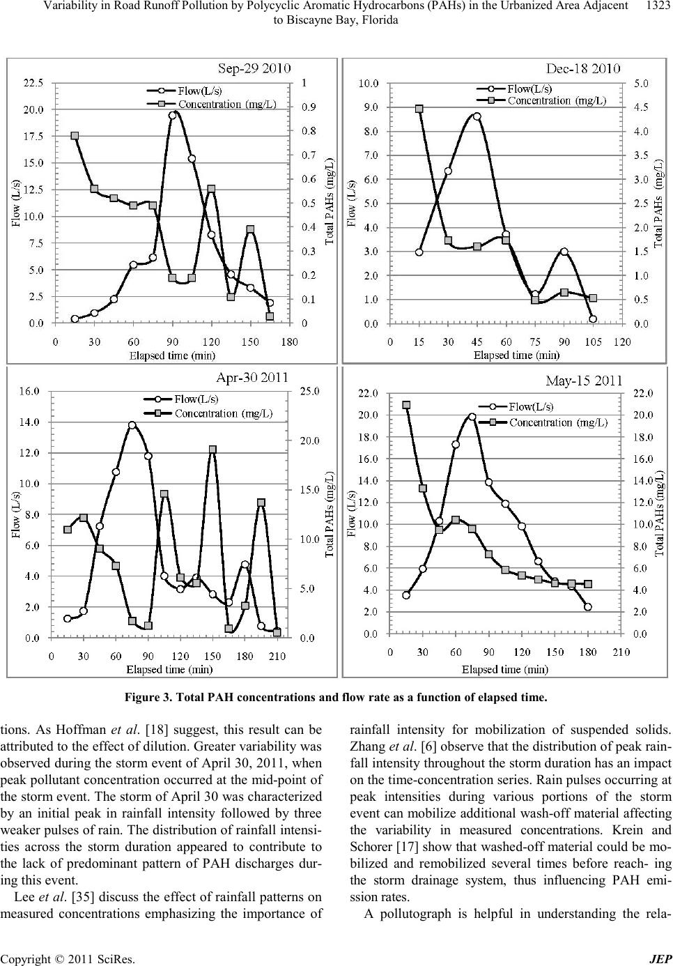

Variability in Road Runoff Pollution by Polycyclic Aromatic Hydrocarbons (PAHs) in the Urbanized Area Adjacent 1323
to Biscayne Bay, Florida
Figure 3. Total PAH concentrations and flow rate as a function of elapsed time.
tions. As Hoffman et al. [18] suggest, this result can be
attributed to the effect of dilution. Greater variability was
observed during the storm event of April 30, 2011, when
peak pollutant concentration occurred at the mid-point of
the storm event. The storm of April 30 was characterized
by an initial peak in rainfall intensity followed by three
weaker pulses of rain. The distribution of rainfall intensi-
ties across the storm duration appeared to contribute to
the lack of predominant pattern of PAH discharges dur-
ing this event.
Lee et al. [35] discuss the effect of rainfall patterns on
measured concentrations emphasizing the importance of
rainfall intensity for mobilization of suspended solids.
Zhang et al. [6] observe that the distribution of peak rain-
fall intensity throughout the storm duration has an impact
on the time-concentration series. Rain pulses occurring at
peak intensities during various portions of the storm
event can mobilize additional wash-off material affecting
the variability in measured concentrations. Krein and
Schorer [17] show that washed-off material could be mo-
bilized and remobilized several times before reach- ing
the storm drainage system, thus influencing PAH emi-
ssion rates.
A pollutograph is helpful in understanding the rela-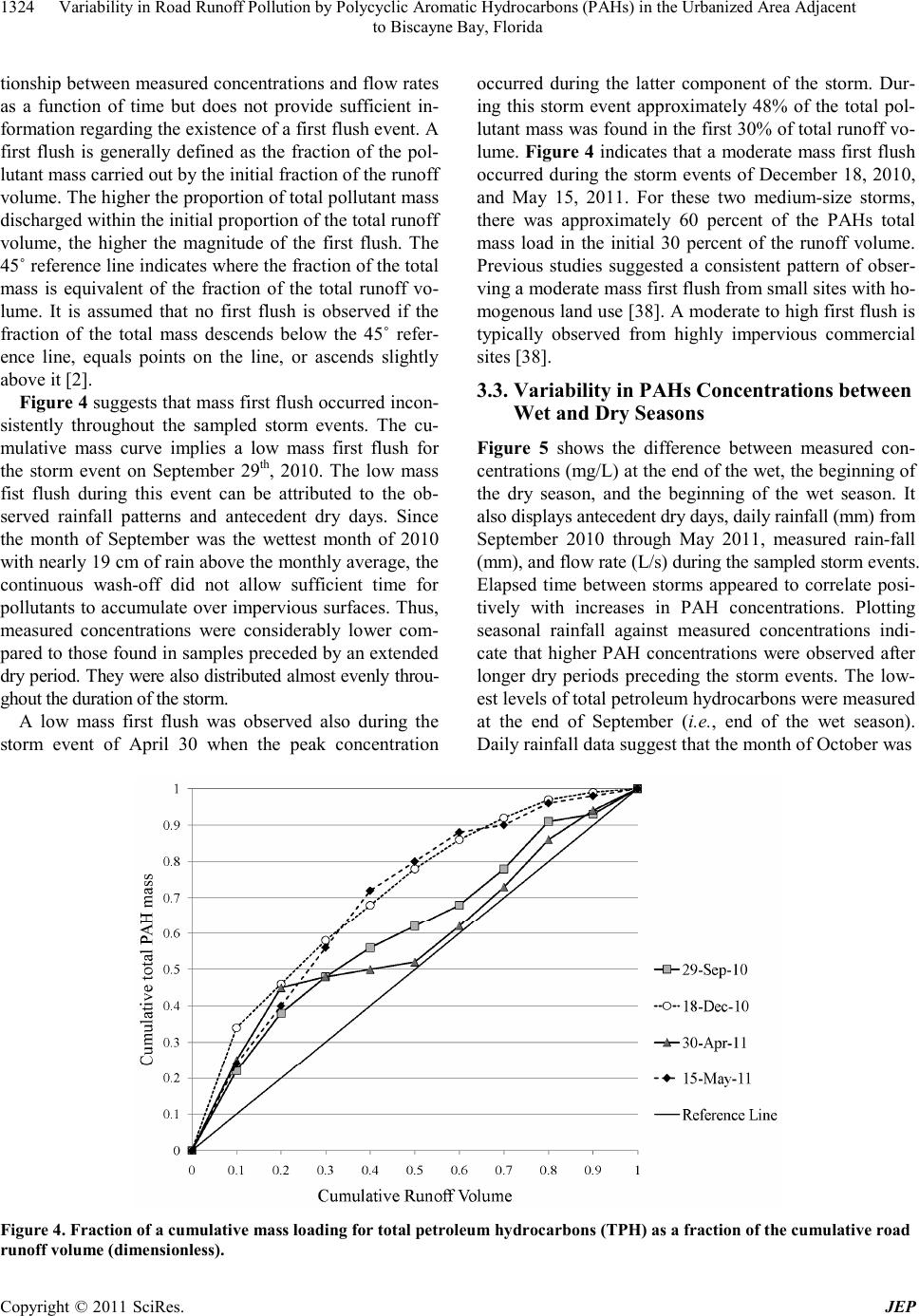

Variability in Road Runoff Pollution by Polycyclic Aromatic Hydrocarbons (PAHs) in the Urbanized Area Adjacent 1324
to Biscayne Bay, Florida
tionship between measured concentrations and flow rates
as a function of time but does not provide sufficient in-
formation regarding the existence of a first flush event. A
first flush is generally defined as the fraction of the pol-
lutant mass carried out by the initial fraction of the runoff
volume. The higher the proportion of total pollutant mass
discharged within the initial proportion of the total runoff
volume, the higher the magnitude of the first flush. The
45˚ reference line indicates where the fraction of the total
mass is equivalent of the fraction of the total runoff vo-
lume. It is assumed that no first flush is observed if the
fraction of the total mass descends below the 45˚ refer-
ence line, equals points on the line, or ascends slightly
above it [2].
Figure 4 suggests that mass first flush occurred incon-
sistently throughout the sampled storm events. The cu-
mulative mass curve implies a low mass first flush for
the storm event on September 29th, 2010. The low mass
fist flush during this event can be attributed to the ob-
served rainfall patterns and antecedent dry days. Since
the month of September was the wettest month of 2010
with nearly 19 cm of rain above the monthly average, the
continuous wash-off did not allow sufficient time for
pollutants to accumulate over impervious surfaces. Thus,
measured concentrations were considerably lower com-
pared to those found in samples preceded by an extended
dry period. They were also distributed almost evenly throu-
ghout the duration of the storm.
A low mass first flush was observed also during the
storm event of April 30 when the peak concentration
occurred during the latter component of the storm. Dur-
ing this storm event approximately 48% of the total pol-
lutant mass was found in the first 30% of total runoff vo-
lume. Figure 4 indicates that a moderate mass first flush
occurred during the storm events of December 18, 2010,
and May 15, 2011. For these two medium-size storms,
there was approximately 60 percent of the PAHs total
mass load in the initial 30 percent of the runoff volume.
Previous studies suggested a consistent pattern of obser-
ving a moderate mass first flush from small sites with ho-
mogenous land use [38]. A moderate to high first flush is
typically observed from highly impervious commercial
sites [38].
3.3. Variability in PAHs Concentrations between
Wet and Dry Seasons
Figure 5 shows the difference between measured con-
centrations (mg/L) at the end of the wet, the beginning of
the dry season, and the beginning of the wet season. It
also displays antecedent dry days, daily rainfall (mm) from
September 2010 through May 2011, measured rain-fall
(mm), and flow rate (L/s) during the sampled storm events.
Elapsed time between storms appeared to correlate posi-
tively with increases in PAH concentrations. Plotting
seasonal rainfall against measured concentrations indi-
cate that higher PAH concentrations were observed after
longer dry periods preceding the storm events. The low-
est levels of total petroleum hydrocarbons were measured
at the end of September (i.e., end of the wet season).
Daily rainfall data suggest that the month of October was
Fig ure 4. Fract ion of a cumulative mass loading f or total petroleum hydrocarbons (TPH) as a fraction of the cumulative road
runoff volume (dimensionless).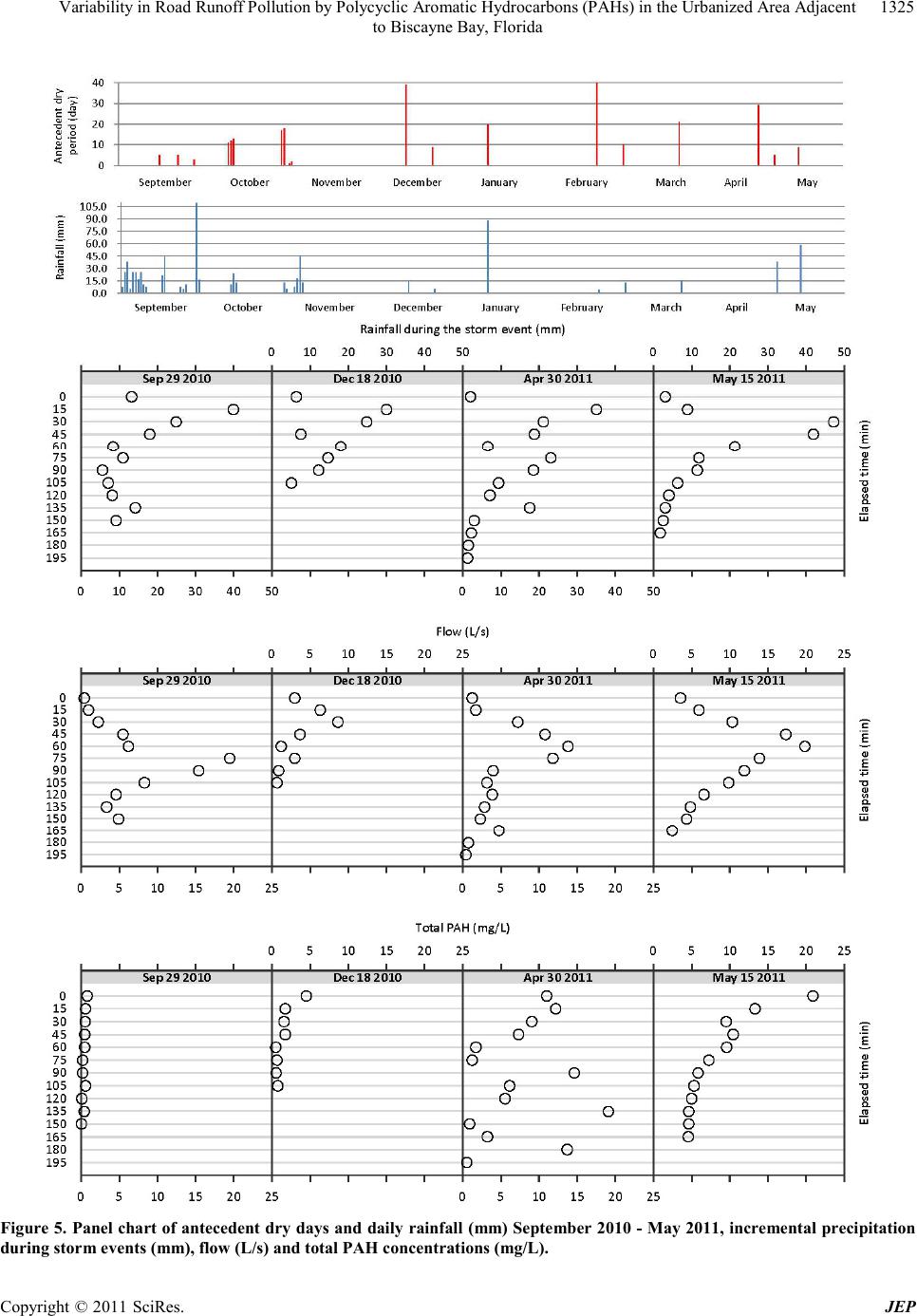

Variability in Road Runoff Pollution by Polycyclic Aromatic Hydrocarbons (PAHs) in the Urbanized Area Adjacent 1325
to Biscayne Bay, Florida
Figure 5. Panel chart of antecedent dry days and daily rainfall (mm) September 2010 - May 2011, incremental precipitation
uring storm events (mm), flow (L/s) and total PAH concentrations (mg/L). d

Variability in Road Runoff Pollution by Polycyclic Aromatic Hydrocarbons (PAHs) in the Urbanized Area Adjacent
to Biscayne Bay, Florida
1326
significantly drier than normal with a deficit of –11.7 cm
below the monthly average, while November and De-
cember recorded deficits of –2.7 and –2.5 cm below the
monthly average, respectively. The rainfall totals for the
months of February and March were again below aver-
age with –4.7 cm and –3.6 cm, respectively. After the
occurrence of relatively dry conditions in October and
November, the samples collected in mid-December con-
tained higher total PAH concentrations. The total PAH
concentrations measured in samples collected in April
and May 2011 after an extended and drier than normal
season were considerably higher suggesting that accu-
mulation of pollutants played a role in increased total
PAH levels. These findings appear to be consistent with
the results of previous studies conducted in climates with
wet/dry seasons. Stein et al. [5] associated increasing
PAH mass-loading rate to longer antecedent dry periods
due to related build-up of pollutants over pervious and
impervious surfaces.
Table 1 shows that the lowest event-based FWMC
(0.310 mg/L) was estimated for the site with higher traf-
fic volume during the storm event of September 30, 2010.
A FWMC of 1.8 mg/L was estimated for the site with the
lower traffic intensity during the storm event of Decem-
ber 18, 2010. Overall, the estimated FWMCs at the end
of the dry season were found to be considerably higher –
5.8 mg/L for the storm event of April 30, 2011 (for the
site with lower traffic intensity) and 8.5 mg/L for the
storm event of May 15, 2011 (for the site with higher
traffic intensity). Table 1 also displays the results from
the estimated partial flow-weighted mean concentrations
for the first 30, 60, 90, 120 and 150 minutes of the storm
event. All sampled storms exhibited a similar pattern of
declining partial FWMCs with each 30-minute interval.
The only exception was the storm of April 30 in which a
sharp increase in the partial FWMC at the beginning of
storm was followed by a sharp decline over the second
interval of 30 minutes, and again an increase in total
PAHs levels over the third and fourth 30-minute intervals.
The partial FWMC at the end of the fifth 30-minute in-
terval for the storm of May 15, 2011 was higher than the
partial FWMCs for the remaining three storm events.
Kendall’s tau testing the concordance between flow-
weighted mean concentrations and antecedent dry days
yielded a Kendall’s tau-a = 0.979 with a p-value = 0.02.
From these results, we can conclude a strong positive
statistically significant correlation between FWMCs and
antecedent dry days. The Kendall rank coefficient was
also used to test the null hypothesis of concordance be-
tween flow-weighted mean concentrations and annual
average daily traffic. The test yielded a Kendall’s tau-a =
–0.33 with a p-value of 0.26. The test statistic did not
show a statistically significant correlation between the two
variables. From these results, we cannot reject the null
hypothesis of mutual independence between FWMCs and
traffic intensity. Higher levels of pollutant accumulation
after a prolonged dry season appear to have a sizeable
effect on PAH FWMCs.
Average seasonal precipitation for the dry and wet sea-
sons was used to calculate the seasonal unit loading rate
for total petroleum hydrocarbons. The end-of wet season
unit loading rate for the road with a higher traffic volume
was 0.589 kg/ha (5.89E-03 kg/km2). The value is lower
than the total PAHs mass-loading rate at the beginning of
the dry season for the road with the lower traffic volume
which was 1.34 kg/ha (1.34E-02 kg/km2). The total PAHs
mass-loading rate at the beginning of the wet season was
8.38 kg/ha (8.38E-02 kg/km2) at the site with lower
AADT counts and 21.57 kg/ha) (2.16E-01 kg/km2) at the
site with higher AADT counts, respectively.
These findings suggest that at the end of the dry sea-
son and the beginning of the wet season higher PAH
mass-loading rate was generated from the site with lower
traffic volume, while at the end of the dry season higher
PAH mass-loading rate was generated at the site with
higher annual average daily traffic counts. The mass-load-
Table 1. Storm flow-weighted meanconcentrations (FWMCs), partial FWMCs at storm durations of 30, 60, 90, 120 and 150
minutes and total PAHs mass-loading rate (kg/km2).
Parameter Storm Event
Sep-29 2010 Dec-18 2010 Apr-30 2011 May-15 2011
Event FWMC (mg/L) 0.310 1.809 5.826 8.491
Partial FWMC30 (mg/L) 0.793 2.353 14.576 16.718
Partial FWMC60 (mg/L) 0.695 1.043 1.934 13.079
Partial FWMC90 (mg/L) 0.289 0.919 7.401 5.978
Partial FWMC120 (mg/L) 0.392 0.452 6.141 4.805
Partial FWMC150 (mg/L) 0.328 0.830 3.884
Total PAHs mass-loading rate (kg/km2) 0.006 0.013 0.084 0.216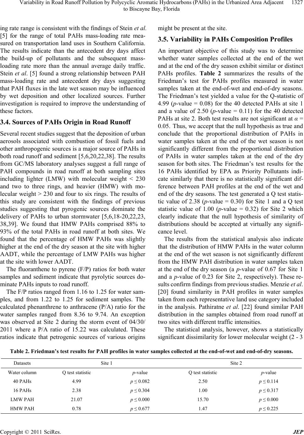

Variability in Road Runoff Pollution by Polycyclic Aromatic Hydrocarbons (PAHs) in the Urbanized Area Adjacent 1327
to Biscayne Bay, Florida
ing rate range is consistent with the findings of Stein et al.
[5] for the range of total PAHs mass-loading rate mea-
sured on transportation land uses in Southern California.
The results indicate than the antecedent dry days affect
the build-up of pollutants and the subsequent mass-
loading rate more than the annual average daily traffic.
Stein et al. [5] found a strong relationship between PAH
mass-loading rate and antecedent dry days suggesting
that PAH fluxes in the late wet season may be influenced
by wet deposition and other localized sources. Further
investigation is required to improve the understanding of
these factors.
3.4. Sources of PAHs Origin in Road Runoff
Several recent studies suggest that the deposition of urban
aerosols associated with combustion of fossil fuels and
other anthropogenic sources is a major source of PAHs in
both road runoff and sediment [5,6,20,22,38]. The results
from GC/MS laboratory analyses suggest a full range of
PAH compounds in road runoff at both sampling sites
including lighter (LMW) with molecular weight < 230
and two to three rings, and heavier (HMW) with mo-
lecular weight > 230 and four to six rings. The results of
this study are consistent with the findings of previous
studies suggesting that pyrogenic sources dominate the
delivery of PAHs to urban stormwater [5,6,18-20,22,23,
38,39]. We found that HMW PAHs comprised 88% to
93% of the total PAHs in road runoff at both sites. We
found that the percentage of HMW PAHs was slightly
higher at the end of the dry season at the site with higher
AADT, while the percentage of LMW PAHs was higher
at the site with lower AADT.
The fluoranthene to pyrene (F/P) ratios for both water
samples and sediment indicate that pyrolytic sources do-
minate PAHs inputs to road runoff.
The F/P ratios ranged from 1.16 to 1.25 for water sam-
ples, and from 1.22 to 1.25 for sediment samples. The
calculated phenanthrene to anthracene (P/A) ratio for the
water samples ranged from 8.36 to 9.74. An exception
was observed at Site 2 during the storm event of 04/30/
2011 where a P/A ratio of 15.22 was calculated. These
ratios indicate that petrogenic sources of various origins
might be present at the site.
3.5. Variability in PAHs Com p ositi on Profiles
An important objective of this study was to determine
whether water samples collected at the end of the wet
and at the end of the dry season exhibit similar or distinct
PAHs profiles. Table 2 summarizes the results of the
Friedman’s test for PAHs profiles measured in water
samples taken at the end-of-wet and end-of-dry seasons.
The Friedman’s test yielded a value for the Q-statistic of
4.99 (p-value = 0.08) for the 40 detected PAHs at site 1
and a value of 2.50 (p-value = 0.11) for the 40 detected
PAHs at site 2. Both test results are not significant at α =
0.05. Thus, we accept that the null hypothesis as true and
conclude that the proportional distribution of PAHs in
water samples taken at the end of the wet season is not
significantly different from the proportional distribution
of PAHs in water samples taken at the end of the dry
season for both sites. The Friedman’s test results for the
16 PAHs identified by EPA as Priority Pollutants indi-
cate similarly that there is no statistically significant dif-
ference between PAH profiles at the end of the wet and
end of the dry seasons. The test generated a Q test statis-
tic value of 2.38 (p-value = 0.30) for Site 1 and a Q test
statistic value of 1.00 (p-value = 0.32) for Site 2 which
clearly indicate that the null hypothesis of similarity of
distributions should be accepted at virtually any signifi-
cance level.
The results from the statistical analysis also indicate
that the distribution of HMW PAHs in the water column
at the end of the wet season is not significantly different
from the HMW PAH distribution in water samples taken
at the end of the dry season (a p-value of 0.67 for Site 1
and a p-value of 0.23 for Site 2, respectively). These re-
sults confirm findings from previous studies. Menzie et al.
[20] found similarity in PAH profiles in water samples
taken from each representative land use category included
in the analysis. Pathiratne et al. [22] found similar PAH
distribution in the samples obtained from road runoff at
two sites with different traffic intensities.
The statistical analysis, however, shows a statistically
significant dissimilarity for lower molecular weight (2 - 3
Table 2. Friedman’s test results for PAH profiles in water samples collected at the end- of-wet and e nd-of-dry seasons.
Datasets Site 1 Site 2
Water column Q test statistic p-value Q test statistic p-value
40 PAHs 4.99 p ≤ 0.082 2.50 p ≤ 0.114
16 PAHs 2.38 p ≤ 0.304 1.00 p ≤ 0.317
LMW PAH 21.07 p ≤ 0.000 15.70 p ≤ 0.000
HMW PAH 0.78 p ≤ 0.677 1.47 p ≤ 0.225

Variability in Road Runoff Pollution by Polycyclic Aromatic Hydrocarbons (PAHs) in the Urbanized Area Adjacent 1328
to Biscayne Bay, Florida
rings) PAHs in water samples. The test generated a Q test
statistic value of 21.07 (p-value = 0.0003) for Site 1), and
a Q test statistic value of 15.70 (p-value = 0.00007) for
Site 2) These results indicate a statistically significant
difference between LMW PAHs profiles at the end of the
wet dry seasons. Possible explanation can be found in the
processes of chemical breakdown of PAHs depending on
their physical and chemical properties, the type of sorp-
tion surfaces (e.g., soil and sediment), and exposure to
photochemical reagents [40]. Several LMW PAH including
anthracene, benzo(a)pyrene, and pyrene are known to be
susceptible to reactions with hydroxyl radicals and are in
most cases degraded faster than the highly hydrophobic
PAHs with four to six fused rings [40].
4. Conclusions
This study investigated PAH contamination in road run-
off with respect to the temporal and spatial distribution of
PAH species. The study found higher PAHs levels in
samples collected at both sites after an extended and drier
than normal dry season. The estimated flow-weighted mean
concentrations for the sampled storm events lead to si-
milar conclusions. The relative magnitude of the esti-
mated PAH mass-loading rates were found to be higher
at the end of the dry season. The results indicated that
higher PAH concentrations measured at the beginning of
the storm event were not always indicative of a first flush.
A storm first flush was found to occur inconsistently
throughout the sampled storm events. The results also
indicated that site characteristics, rainfall patterns and
intensity, flow volume and antecedent dry period af-
fected the mobilization and remobilization of pollutants
and therefore played a role in PAHs delivery to receiving
waters. The importance of the length of time between
subsequent storm events available for pollutants to build
up on impervious surfaces, identified by previous studies,
was confirmed by this investigation.
The effect of the annual average daily traffic on PAHs
concentrations in water samples requires further investi-
gation. The continuous accumulation and wash-off of po-
llutants appeared to affect measured concentrations more
than the traffic intensity. We found higher total PAHs con-
centrations in runoff samples at the site with the lower
traffic intensity compared to the site with heavier traffic
at the beginning of the dry season. Conversely, we found
lower total PAH concentrations in runoff samples at the
same site at the beginning of the wet season compared to
the PAH levels at the site with higher AADT counts.
Zhang et al. [6] reported higher PAH concentrations at
sites with lower traffic volumes and suggested that fac-
tors beyond the level of service such seasonality in rain-
fall patterns and site characteristics exerted strong in-
fluence on the level of PAHs concentrations in road run-
off samples. A limitation of this study is that it does not
account for the effect of the BMPs and pretreatment mea-
sures that could reduce PAH discharges before they
reach receiving waters. There appears to be a need for fu-
ture studies evaluating the feasibility of treating the first
flush fraction of the storm after prolonged dry periods.
5. Acknowledgments
This study was supported through a grant by the FAU
Environmental Sciences Everglades Fellowship Program
funded by the National Park Service under Task Agree-
ment J5284-09-0004, Cooperative Agreement H5000-06-
0103. The findings and opinions reported are those of the
authors and do not necessarily reflect the views of the
funding agencies. We wish to acknowledge the contribu-
tion of Sarah Bellmund and Brigette Castro from Bis-
cayne National Park who guided us in refining the meth-
odology and selecting the sampling sites. We also ac-
knowledge the valuable support of Adolfo Fernandez and
Ingrid Ley from the Department of Chemistry & Bio-
chemistry and Southeast Environmental Research Center
(SERC) at Florida International University; Ricardo Sa-
lazar and Larry W. Minor of the Florida Department of
Transportation, District 6; and Steven Blair and Forest
Shaw of the Department of Environmental Resources
Management of Miami-Dade County.
REFERENCES
[1] I. D. Bossert and R. Bartha, “Structure-Biodegradability
Relationships of Polycyclic Aromatic Hydrocarbons in
Soil,” Bulletin of Environmental Contamination and Toxi-
cology, Vol. 37, No. 1, 1986, pp. 490-495.
doi:10.1007/BF01607793
[2] M. Kayhanian and M. K. Stenstrom, “First-Flush Charac-
terization for Stormwater Treatment,” Stormwater, 2008.
http://www.stormh2o.com/march-april-2008/pollutants-ru
n-off.aspx
[3] L. H. Kim, M. Kayhanian, K.-D. Zoh and M. K. Sten-
strom, “Modeling of Highway Stormwater Runoff,” Sci-
ence of the Total Environment, Vol. 348, No. 1-3, 2005,
pp. 1-18. doi:10.1016/j.scitotenv.2004.12.063
[4] J. Soller, J. Stephenson, K. Olivieri, J. Downing and A.
W. Olivieri, “Evaluation of the Seasonal Scale First Flush
Pollutant Loading and Implications for Urban Runoff Ma-
nagement,” Journal of Environmental Management, Vol.
76, 2005, pp. 309-318.
[5] E. D. Stein, L. L. Toefenthaler and K. Schiff, “Water-
shed-Based Sources of Polycyclic Aromatic Hydrocar-
bons in Urban Stormwater,” Environmental Toxicology
and Chemistry, Vol. 25, No. 2, 2006, pp. 373-385.
[6] W. Zhang, S. Zhang, D. Yue, C. Wan, Y. Ye and X. Wang,
“Characterization and Loading Estimation of Polycyclic

Variability in Road Runoff Pollution by Polycyclic Aromatic Hydrocarbons (PAHs) in the Urbanized Area Adjacent 1329
to Biscayne Bay, Florida
Aromatic Hydrocarbons in Road Runoff from Urban Re-
gions of Beijing, China,” Environmental Toxicology and
Chemistry, Vol. 27, No. 1, pp. 31-37.
doi:10.1897/07-030.1
[7] C. M. Teaf, D. J. Covert and S. R. Kothur, “Urban Poly-
cyclic Aromatic Hydrocarbons (PAHS): A Florida Per-
spective,” Proceedings of the Annual International Con-
ference on Soils, Sediment, Water and Energy, Vol. 13,
No. 1, 2008, Article 23.
[8] D. J. McKenzie and G. A. Irwin, “Water-Quality As-
sessment of Stormwater Runoff from a Heavily Used Ur-
ban Highway Bridge in Miami, Florida,” USGS Water
Resources Investigations 83-4153 (FHWA/FL/BMR-84-
270), 1983.
[9] E. F. Corcoran, M. S. Brown, F. R. Baddour, S. A. Cha-
sens and A. D. Freay, “Biscayne Bay Hydrocarbon Stu-
dy,” NOAA Technical Memorandum NOS NCCOS 9,
University of Miami RSMAS TR 2005-01, Coastal and
Estuarine Data Archeology and Rescue Program, 1983.
[10] K. H. Haag, R. L. Miller, L. A. Bradner and D. S. Mc-
Culloch, “Water-Quality Assessment of Southern Florida:
An Overview of Available Information on Surface and
Ground-Water Quality and Ecology,” US Geological Sur-
vey, Water-Resources Investigations Report 96-4177, Tal-
lahassee, 1996.
[11] A. Y. Cantillo, G. G. Lauenstein and T. P O’Connor,
“Mollusc and Sediment Contaminant Levels and Trends
in South Florida Coastal Waters,” Marine Pollution Bul-
letin, Vol. 34, No. 7, 1997, pp. 511-521.
doi:10.1016/S0025-326X(96)00152-X
[12] V. G. Caccia and J. N. Boyer, “Spatial Patterning of Wa-
ter Quality in Biscayne Bay, Florida as a Function of Land
Use and Water Management,” Marine Pollution Bulletin,
Vol. 50, No. 11, 2005, pp. 1416-1429.
doi:10.1016/j.marpolbul.2005.08.002
[13] T. L. Seal, F. D. Calder, G. M. Sloane, S. J. Schropp and
H. L. Windom, “Florida Coastal Sediment Contaminants
Atlas,” Florida Department of Environmental Protection,
Tallahassee, 1994.
[14] E. R. Long, G. Sloane, G. Scott, B. Thompson, R. S. Carr,
J. Biedenbach, T. Wade, B. Presley, K. Scott, C. Mueller,
G. Breken-Fols, B. Albrecht, J. W. Anderson and G. T.
Chandler, “Magnitude and Extent of Chemical Contami-
nation and Toxicity in Sediments of Biscayne Bay and
Vicinity,” NOAA Technical Memorandum 141, 2000.
[15] E. R. Long, M. J. Hameedi, G. M. Sloane and L. B. Read,
“Chemical Contamination, Toxicity, and Benthic Com-
munity Indices in Sediments of the Lower Miami River
and Adjoining Portions of Biscayne Bay, Florida,” Estu-
aries, Vol. 25, No. 4A, 2002, pp. 622-637.
doi:10.1007/BF02804895
[16] M. K. Stenstrom and M. Kayhanian, “First Flush Phe-
nomenon Characterization,” CTSW-RT-05-73-02.6, Pre-
pared for the California Department of Transportation
Division of Environmental Analysis, 2005.
[17] A. Krein and M. Schorer, “Road Runoff Pollution by
Polycyclic Aromatic Hydrocarbons and Its Contribution to
River Sediments,” Water Research, Vol. 34, No. 16, 2000,
pp. 4110-4115.
[18] E. J. Hoffman, G. L. Mills, J. S. Latimer and J. G. Quinn,
“Urban Runoff as a Source of Polycyclic Aromatic Hy-
drocarbons to Coastal Waters,” Environmental Science
and Technology, Vol. 18, No. 8, 1984, pp. 580-587.
doi :1 0. 10 21 /e s001 26 a0 03
[19] B. Ngabe, T. F. Bidleman and G. I. Scott, “Polycyclic
Aromatic Hydrocarbons in Storm Runoff from Urban and
coastal South Carolina,” The Science of the Total Envi-
ronment, Vol. 255, No. 1-3, 2000, pp. 1-9.
doi:10.1016/S0048-9697(00)00422-8
[20] C. A. Menzie, S. S. Hoeppner, J. J. Cura, J. S. Freshman
and E. N. LaFrey, “Urban and Suburban Storm Water
Runoff as a Source of Polycyclic Aromatic Hydrocarbons
(PAHs) to Massachusetts Estuarine and Coastal Envi-
ronments,” Estuaries, Vol. 25, No. 2, 2002, pp. 165-176.
doi:10.1007/BF02691305
[21] H. M. Hwang and G. D. Foster, “Characterization of
Polycyclic Aromatic Hydrocarbons in Urban Stormwater
Runoff Flowing into the Tidal Anacostia River,” Envi-
ronmental Pollution, Vol. 140, No. 3, 2006, pp. 416-426.
doi:10.1016/j.envpol.2005.08.003
[22] K. A. S. Pathiratne, O. C. P. de Silva, D. Hehemann, I.
Atkinson and R. Wei, “Occurrence and Distribution of
Polycyclic Aromatic Hydrocarbons (PAHs) in Bolgoda
and Beira Lakes, Sri Lanka,” Bulletin of Environmental
Contamination and Toxicology, Vol. 79, No. 2, 2007, pp.
135-140. doi:10.1007/s00128-007-9092-z
[23] E. J. Hoffman, J. S. Latimer, C. D. Hunt, G. L. Mills and
J. G. Quinn, “Stormwater Runoff from Highways,” Water,
Air, and Soil Pollution, Vol. 25, No. 4, 1985, pp. 349-
364. doi:10. 10 07/B F0 02 83 78 8
[24] E. Hong, E. A. Seagren and A. P. Davis, “Sustainable Oil
and Grease Removal from Synthetic Stromwater Runoff
Using Bench-Scale Bio-Retention Studies,” Water Envi-
ronment Research, Vol. 78, No. 2, 2006, pp. 141-155.
doi:10.2175/106143005X89607
[25] J. J. Sansalone and S. G. Buchberger, “Partitioning and
First Flush of Metals in Urban Roadway Stormwater,”
Journal of Environmental Engineering, Vol. 123, No. 2,
1997, pp. 134-143.
doi:10.1061/(ASCE)0733-9372(1997)123:2(134)
[26] J.-L. Bertrand-Krajewski, G. Chebbo and A. Saget, “Dis-
tribution of Pollutant Mass vs Volume in Stormwater
Discharges and the First Flush Phenomenon,” Water Re-
search, Vol. 32, No. 8, 1998, pp. 2341-2356.
doi:10.1016/S0043-1354(97)00420-X
[27] A. Deletic, “The First Flush Load of Urban Surface Run-
off,” Water Research, Vol. 32, No. 8, pp. 2462-2470.
doi:10.1016/S0043-1354(97)00470-3
[28] M. Kayhanian, A. Singh, C. Suverkropp and S. Borrum,
“Impact of Annual Average Daily Traffic on Highway
Pollutant Concentrations,” Journal of Environmental En-
gineering, Vol. 129, No. 11, 2003, pp. 975-990.
doi:10.1061/(ASCE)0733-9372(2003)129:11(975)

Variability in Road Runoff Pollution by Polycyclic Aromatic Hydrocarbons (PAHs) in the Urbanized Area Adjacent
to Biscayne Bay, Florida
1330
[29] J. H. Lee and K. W. Bang, “Characterization of Urban
Stormwater Runoff,” Water Research, Vol. 34, No. 6,
2000, pp. 1773-1780.
doi:10.1016/S0043-1354(99)00325-5
[30] B. Suderman and N. H. Marcus, “The Effects of Orimul-
sion and Fuel Oil #6 on the Hatching Success of Copepod
Resting Eggs in the Seabed of Tampa Bay, Florida,” En-
vironmental Pollution, Vol. 120, No. 3, 2002, pp. 787-
795.
[31] J. Obeysekera, J. Browder, L. Horning and M. A. Harwell,
“The Natural South Florida System I: Climate, Geology,
and Hydrology,” Urban Ecosystems, Vol. 3, No. 3-4, 1999,
pp. 223-244. doi:10.1023/A:1009552500448
[32] National Oceanic and Atmospheric Administration—Na-
tional Weather Service (NOAA-NWS), “Duration of Sum-
mer Season in South Florida,” Miami-South Florida Wea-
ther Forecast Office, Miami, 2010.
http://www.srh.noaa.gov/mfl/summer_season
[33] Florida Department of Transportation FDOT, “Geographic
Information System (GIS): GIS Shapefiles,” 2010.
http://www.dot.state.fl.us/planning/statistics/gis/tra fficdata.
shtm
[34] US Environmental Protection Agency (USEPA), “NPDES
Storm Water Sampling Guidance Document,” EPA 833-8-
92-001, Office of Water, Washington DC, 1992.
[35] J. H. Lee, S. L. Lau, M. Kayhanian and M. K. Stenstrom,
“Seasonal First Flush Phenomenon of Urban Stormwater
Discharges,” Water Research, Vol. 38, No. 19, 2004, pp.
4153-4163. doi:10.1016/j.watres.2004.07.012
[36] P. Leftwich, D. Zierden and M. Griffin, “Monthly Cli-
mate Summaries for Florida,” Florida Climate Center,
Office of the State Climatologist, Florida State University,
Tallahassee, 2009-2011.
[37] J. H. Lee, K. W. Bang, L. H. Ketchum, J. S. Choe and M.
J. Yu, “First Flush Analysis of Urban Storm Runoff,” Sci-
ence of the Total Environment, Vol. 293, No. 1-3, 2002,
pp. 163-175. doi:10.1016/S0048-9697(02)00006-2
[38] E. D. Stein, L. L. Tiefenthaler and K. C. Schiff, “Com-
parison of Stromwater Pollutant Loading by Land Use
Type,” Southern California Coastal Water Research Pro-
ject, AR08-015-027, 2008.
http://www.sccwrp.org/Documents/AnnualReports/Brows
eAllAnnualReports/2008AnnualReport.aspx.
[39] M. K. Stenstrom, G. S. Silverman and T. A. Bursztynsky,
“Oil and Grease in Urban Stormwaters,” ASCE Journal of
the Environmental Engineering Division, Vol. 110, No. 1,
1984, pp. 58-72.
doi:10.1061/(ASCE)0733-9372(1984)110:1(58)
[40] S. Jonsson, Y. Persson, S. Frankki, B. van Bavel, S.
Lundstedt, P. Haglund and M. Tysklind, “Degradation of
Polycyclic Aromatic Hydrocarbons (PAHs) in Contami-
nated Soils by Fenton’s Reagent: A Multivariate Evalua-
tion of the Importance of Soil Characteristics and PAH
Properties,” Journal of Hazardous Materials, Vol. 149,
No. 1, 2007, pp. 86-96.