Journal of Analytical Sciences, Methods and Instrumentation, 2011, 1, 9-18
doi:10.4236/jasmi.2011.12002 Published Online December 2011 (http://www.SciRP.org/journal/jasmi)
9
Handling Observations with Low Interrater
Agreement Values
Gensheng (Jason) Liu, Mohammad M. Amini, Emin Babakus, Marla B. Royne Stafford
Department of Marketing & Supply Chain Management, University of Memphis, Memphis, USA.
Received October 30th, 2011; revised November 17th, 2011; accepted November 29th, 2011.
ABSTRACT
Considerable research has been conducted on how interrater agreement (IRA) should be established before data can be
aggregated from the individual rater level to the organization level in survey research. However, little is known about
how researchers should treat the observations with low IRA values fail to meet the suggested standard. We seek to an-
swer this question by investigating the impact of two factors (the relationship strength and the overall IRA level of a
sample) on the IRA decision. Using both real data from a service industry and simulated data, we find that both factors
affect whether a researcher should include or exclude observations with low IRA values. Based on the results, practical
guidelines on when to use the entire sample are offered.
Keywords: Interrater Agreement, Aggregation, Survey Research
1. Introduction
In survey research, using a single respondent to represent
an organization is vulnerable to single-rater bias [1,2];
therefore, multiple raters are recommended. When multi-
ple raters are used, a certain degree of agreement must be
established before the responses can be aggregated to the
organization level. Interrater agreement (IRA) refers to the
absolute consensus in scores assigned by multiple raters
to one or more targets. Estimates of IRA are used to ad-
dress whether scores furnished by different raters are in-
terchangeable or equivalent [3,4].
Previous research has suggested various measures of
IRA. The most widely used one is the rWG index pro-
posed by James et al. [4,5]. Values of 0.7 have been used
as the traditional cutoff value denoting high versus low
IRA using the rWG index [6,7]. Lebreton et al. [6] inter-
pret rWG as the proportional reduction in error variance. A
value of 0.7 suggests a 70% reduction in error variance
and that just 30% of the observed variance among judges’
ratings should be credited to random responding.
Since rWG was first introduced, researchers have ad-
dressed various related issues [3,8-12], but little attention
has been paid to dealing with the observations that have
low rWG values, with only one noticeable exception. Le-
Breton and Senter [3] suggest that researchers examine
the magnitude and pattern of rWG values and state that if
only 5% of values are below the cutoff value, it is proba-
bly justified to use the entire sample of rated targets. Their
statement, however, is rather vague, and no theoretical or
empirical justification is provided for the suggested guide-
line of 5%. In addition, they fail to address what resear-
chers should do if more than 5% of the rWG values are
below the cutoff value. Hence, it is still largely an unan-
swered question in the literature.
Our aim is to address this issue with the current study.
Specifically, we investigate when one can use the average
value of rWG, which is referred to as RWG, to assess whether
or not to include the entire sample, and when one has to
examine rWG of each individual unit of analysis and de-
termine if it should be included in the data analysis. In
other words, we want to find out when we shall start look-
ing at the trees instead of the forest regarding IRA.
2. Background and Research Questions
2.1. rWG as a Measure of IRA
When there is a single target or a single variable:
2
2
1X
WG
E
S
r

=-
where is the observed variance across respondents,
and
2
X
S
2
E

is the variance obtained from a theoretical null
distribution representing a complete lack of agreement
among raters (totally random). When a construct has more
than one parallel measurement item, the index becomes

Handling Observations with Low Interrater Agreement Values
10
()
2
2
22
22
1
1
j
E
WG J
j
j
E
E
S
J
rSS
J



æö
÷
ç÷
ç-÷
ç÷
ç÷
èø
=æö
÷
ç÷
ç-+
÷
ç÷
ç÷
èø
where J is the number of items in the construct, 2
j
S is
the mean of the response variances across items.
The rWG index is widely adopted in various fields such
as services marketing [13], strategic management [14], or-
ganizational behavior [15], and operations management
[16]. 0.7 has been used as the cutoff value denoting whether
IRA is established while using the rWG index [6,7]. rWG is
calculated for each object (observation, unit of analysis,
usually organization) in a survey sample. Theoretically,
for any organization with an rWG below 0.7, aggregation
of the data across raters is not justified. However, in
checking IRA of their data, most researchers calculate
the mean rWG value of all observations in their data set,
which is labeled as RWG.
WG
WG
r
Rn =å,
where n is the sample size, or the number of units (or-
ganizations) in the sample.
If RWG is above 0.7, they will conclude that IRA is
achieved on the entire data set. Therefore, they will ag-
gregate the data on each observation, and subsequently
use all observations to conduct data analysis [17,18]. The
original papers introducing the rWG indices [4,5] have
been cited more than 700 times in different fields ranging
from strategic management to nursing [3]. However, a
review of the services marketing literature revealed that
very few studies excluded observations with low rWG
values [19,20]. Rather, most studies used data on all ob-
servations once RWG was found above 0.7. In some cases,
RWG values as low as 0.50 [21] were deemed acceptable.
Because RWG is the mean of rWG across all observations,
even with some very low rWG values, RWG could still meet
the suggested standard of 0.7. Therefore, a high RWG
value does not guarantee that IRA is achieved across all
units of analysis, and the approach presented above is
problematic. Simply having a mean value RWG above the
0.7 threshold cannot justify data aggregation for those
units that have lower rWG values. Instead, the aggregation
of data on each unit of analysis should be justified based
on the individual rWG of that specific unit.
Yet little research has been conducted on how to han-
dle the observations that have low rWG values. Hence, the
question remains whether they should be excluded from
the data analysis, using only those observations with high
rWG, or whether all observations should be used as long
as their average, RWG, is above 0.7, a practical approach
adopted by most researchers. Although LeBreton and
Senter [3] suggest that aggregation is justified if only 5%
of rWG values are below the 0.7 threshold, no theoretical
or empirical support is provided for this assertion. There-
fore, it remains an unanswered question in the literature,
and one that we seek to answer in this paper. In doing so,
we examined the potential impact of two factors on the
IRA decision: relationship strength and overall IRA level
of the sample.
2.2. Factors That Potentially Affect the IRA
Decision
A number of different factors such as model complexity,
number of items in a construct, and factor loading struc-
ture of a construct potentially affect whether RWG is ade-
quate for inclusion of all observations. We limit the scope
of this study to two of these factors. The first is the strength
of the investigated relationship. The stronger the relation-
ship between two variables, the more robust it is to the
working sample, and the less difference there will be be-
tween parameter estimates using the entire sample versus
using only those observations with high IRA values. That
is, when the relationship between two variables is very
strong, using all data or only the valid data (those obser-
vations with rWG above 0.7) likely makes little difference.
When the relationship between two variables is fairly
weak, better results may be realized if only the valid data
are used.
The second factor that likely affects the decision is the
overall magnitude of IRA, as represented by RWG itself.
As RWG gets higher, the portion of the sample with low
rWG values decreases, so the difference between using the
complete sample and using only those observations with
high IRA values also decreases. When RWG is very high
(e.g., above 0.85), using only the valid data is probably
as good as using all data. However, when RWG is fairly
low, the invalid data might cause too much noise in the
analysis, suggesting that only the valid data should be used.
To the best of our knowledge, this is the first study to
address the issue of whether RWG is adequate for the in-
clusion of all observations. To date, none of the potential
factors have been examined before, including the two
factors we investigate in this study. Findings from this
study have the potential to offer guidelines for research-
ers to determine when to aggregate and use the entire
sample, and when only observations with high enough
rWG values should be used.
3. Research Design
To address these issues, we utilized two different approa-
ches because triangulation enhances the validity of research
results and helps develop a holistic understanding of the
phenomena of interest [1]. The fist approach used actual

Handling Observations with Low Interrater Agreement Values11
data which included two relationships among three vari-
ables that are well established in the services marketing
literature; thus, the only purpose of the analyses was to
answer questions about IRA. In addition, this data set
employs multiple raters. Analysis of this real data should
provide an initial sense of the phenomenon under inves-
tigation.
In the second approach, we used data generated through
simulation. Simulation allowed us to generate multiple
data sets with varying levels of relationship strength and
varying levels of RWG, something not possible with real
data. This approach enabled us to examine the impact of
these two factors in the aggregation decision.
For both data sets, we fitted each model twice. In the
first model, we used the entire sample. In the second model,
we used just a partial sample of those observations with
rWG above 0.7 on both constructs in the relationship. We
then compared the differences between the results. The
rationale is that the aggregated data are valid on observa-
tions with both rWG values above 0.7, but not valid on
observations with either rWG value below 0.7. If no sig-
nificant differences were found between these two ana-
lyses, aggregating the rater level data onto the organiza-
tion level with all units of analysis was justified. How-
ever, if significant differences were found between these
two analyses, under that specific condition, the researcher
should not aggregate data on all units of analysis. Rather,
they should only use those units with rWG above 0.7.
3.1. Analysis with Real Data
As noted, the real data included well-established rela-
tionships in the services marketing literature, and we used
two relationships among three variables to examine the
research questions about IRA. In the services marketing
literature, it is widely acknowledged that the server’s in-
teraction quality with the customer greatly influences both
the customer’s perceived value of the service [22,23] and
the customer’s satisfaction level [24,25]. Therefore, we
chose interaction quality, perceived value, and customer
satisfaction as the variables of interest, and investigate
the two relationships as shown in Figure 1.
Because these well-established relationships are very
strong, the analysis was able to focus solely on the im-
pact of IRA decisions on the relationships. Because we
Figure 1. Relationships in real data analysis.
wanted to keep the relationship simple to analyze, focus-
ing only on the impact of the IRA decisions, we investi-
gated the two relationships separately rather than putting
them together in one combined model. Each of the three
variables was measured with a multi-item scale. Two types
of Likert scales, 7-point and 10-point, were used to avoid
common method bias. All measures were adapted from
established scales in previous literature, and are included
in Appendix A.
Data were collected via mail questionnaires from ran-
domly selected customers of a national bank in New Zea-
land who were given assurance of confidentiality and
anonymity. Respondents were asked to rate their service
experience with one specific bank branch. Of the 2500
questionnaires mailed, 872 were returned yielding a re-
sponse rate of 34.9%. A total of 51 bank branches were
rated by these customers, with each branch rated by an
average of 11.2 customers. When we aggregated the data
from individual customer level to the bank branch level,
the RWG values for the three scales were 0.853, 0.767, and
0.842, respectively.
We analyzed two structural equation models to test the
two relationships. Each model was fitted twice—first with
the entire sample and then with a partial sample of those
bank branches with rWG above 0.7 on both constructs in
the relationship. Results of these analyses are presented
in Table 1.
The first relationship examined is the one between in-
teraction quality and perceived value; 64.7% of the bank
branches have a rWG above 0.7 on both constructs. How-
ever, the model fit indices between the full sample and
the partial sample are slightly different. The standardized
path coefficient for this relationship is 0.613 on the full
sample and 0.761 on the partial sample, and although
both are significant at p < 0.001, the relationship appears
stronger when observations with rWG below 0.7 are not
included in the analysis.
Table 1. Real data analysis results.
Interaction quality
Perceived value
Interaction quality
Customer satisfaction

Full dataPartial data Full data Partial data
Sample size 51 33 (64.7%) 51 42 (82.4%)
Chi-square 47.63 38.65 39.40 38.98
Degree of freedom19 19 26 26
Normed Chi-square2.507 2.034 1.515 1.499
NFI 0.902 0.888 0.938 0.924
CFI 0.937 0.938 0.978 0.973
RMSEA 0.174 0.180 0.102 0.110
Std coefficient 0.613 0.761 0.819 0.840
p
-value <0.001 <0.001 <0.001 <0.001

Handling Observations with Low Interrater Agreement Values
12
The second relationship investigated is between inter-
action quality and customer satisfaction. Because both
constructs have very high RWG (above 0.8), fewer bank
branches actually have an rWG below 0.7 on either of the
constructs, and 82.4% of the 51 bank branches (42) have
an rWG above 0.7 on both constructs. As a result, the
model fit statistics between the full sample and the partial
sample are very close. In addition, the standardized path
coefficient (Gamma) of the relationship is 0.819 for the
full sample and 0.840 for the partial sample, both very
high and very close to each other.
In comparing the two relationships, not only did the
second relationship have a higher RWG on the constructs,
but the relationship between the two variables was
stronger than the first one (Gamma = about 0.8 compared
to about 0.6). These results suggest that IRA decisions
may be more critical for the first relationship because the
results from the full sample as compared to the partial
sample differ to a greater extent. However, because we
cannot control the strength of the underlying relationship
or the magnitude of RWG with the real data, we are unable
to separate the effects of these two factors.
3.2. Analysis with Simulated Data
To separate the effects of the strength of the underlying
relationship and the magnitude of RWG, we used simu-
lated data as a secondary approach to answer the research
questions.
3.2.1. Dat a Generation
With simulated data, the analysis focused on the rela-
tionship between two hypothetical latent variables, ξ and
η. In this case, we assume each of the two constructs has
four measurement items, X1, X2, X3, X4 for ξ, and Y1,
Y2, Y3, Y4 for η. The model is shown in Figure 2.
We used simulation to generate multiple hypothetical
data sets for these two variables with the following spe-
cifications: 1) The sample size was set to be 250, which
is large enough for structural equation modeling analysis
[26]. 2) The response scale was a seven-point Likert scale.
3) For each unit of analysis (organization), there were five
raters. 4) The standardized item loading coefficients for
X1, X2, X3 and X4 on the construct ξ were set to be 0.72,
0.74, 0.76, and 0.80 respectively. The same coefficients
Figure 2. Hypothetical structural model.
apply to the loading of Y1, Y2, Y3 and Y4 onto the con-
struct η. These coefficients were chosen to ensure that at
least 50% (square of the standardized item loading coef-
ficients) of the variance in the measurement items is ex-
plained by the underlying construct. In other words, the
measurement items are all reliable indicators of their
respective underlying constructs. This allows an exclu-
sive focus on our real interest, the structural link between
ξ and η.
Because the magnitude of the difference may depend
on the strength of the relationship and the overall magni-
tude of IRA, we controlled these two factors when gen-
erating the samples. To control the relationship strength
between the latent variables, we chose five levels of Gamma:
0.1, 0.3, 0.5, 0.7, and 0.9. At each level of Gamma, we
had 10 different target levels of RWG for both ξ and η:
0.50, 0.55, 0.60, 0.65, 0.70, 0.75, 0.80, 0.85, 0.90, and
0.95. Empirical experience tells us that when RWG is be-
low 0.50, a significant portion (usually above 80%) of
the observations have rWG values below 0.7, which will
almost inevitably affect the analysis. Therefore, we only
chose levels of RWG above 0.50.
For each Gamma and target RWG combination, we
generated five random samples. These five samples have
exactly the same mean responses, but differ in the rWG
value of each observation. Because we have five levels
of Gamma and ten levels of target RWG, the total number
of samples generated is 5 × 10 × 5 = 250. The detailed si-
mulation process is described in Appendix B.
3.2.2. Dat a Analysis
Using Amos (Version 7.0), we tested the structural equa-
tion model shown in Figure 2 with each of the 250 sam-
ples. The analysis was conducted twice with each sample.
The first analysis was conducted on the full sample of
250 observations, while the second analysis was conducted
on a partial sample that had observations with rWG values
above 0.7 on measures of both ξ and η. A total of 500
analyses were conducted. For each analysis, we recorded
the standardized path coefficient (Gamma) between ξ and
η and the p-value corresponding to it.
Because we conducted the analysis twice with each
sample, it was important to determine which of the two
analyses provided a better estimate of the true population
Gamma. Note that the data sets we generated are not raw
responses, but aggregated responses across the raters of
each target. For the aggregated data to be valid, IRA should
be established first. For observations with low IRA val-
ues (rWG below 0.7), the aggregation itself is not justified.
When comparing a full sample with its corresponding
partial sample, we believe that the partial sample has a
Gamma value that is closer to the true value because data
aggregation is valid on all observations in the partial sample.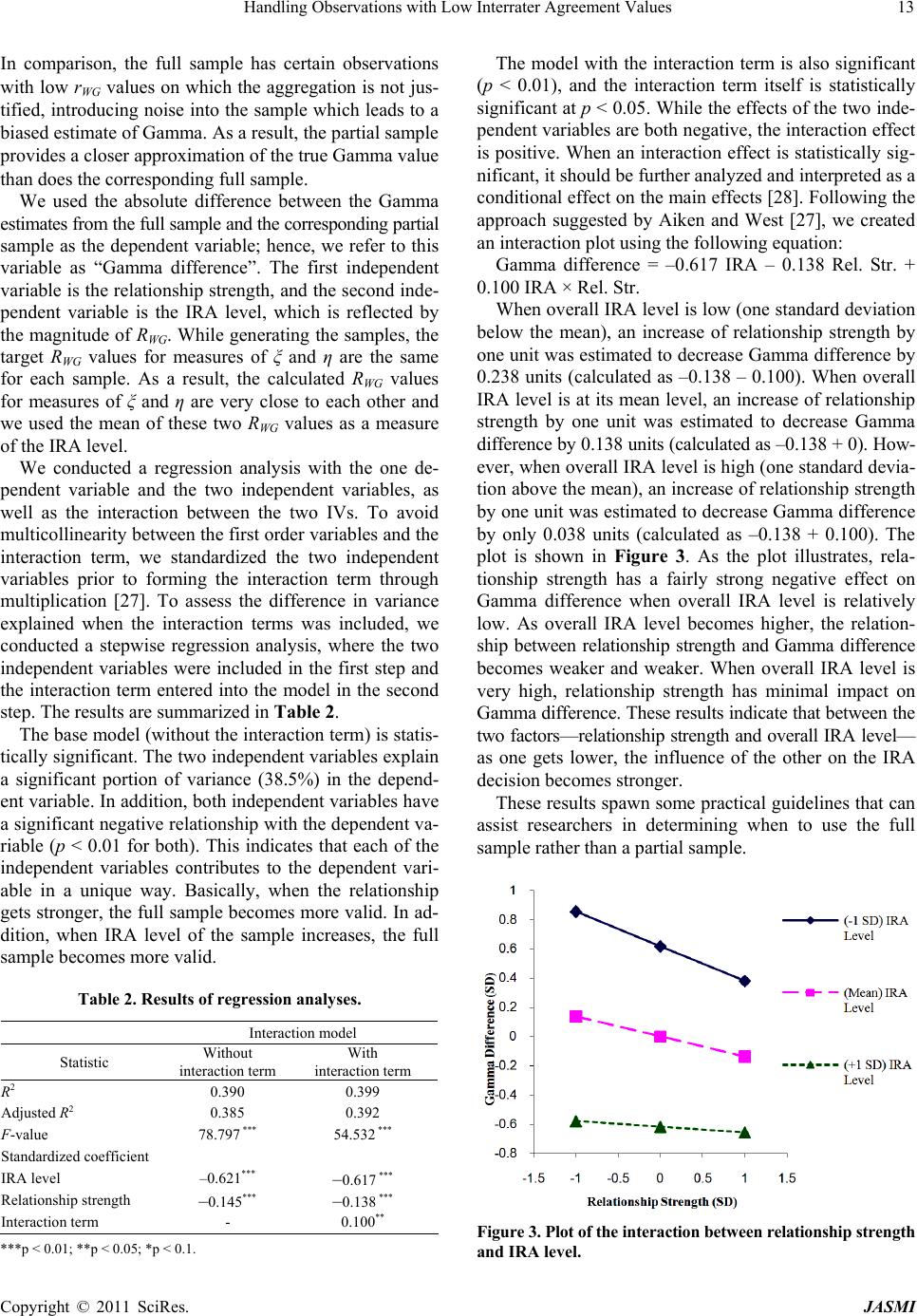

Handling Observations with Low Interrater Agreement Values13
In comparison, the full sample has certain observations
with low rWG values on which the aggregation is not jus-
tified, introducing noise into the sample which leads to a
biased estimate of Gamma. As a result, the partial sample
provides a closer approximation of the true Gamma value
than does the corresponding full sample.
We used the absolute difference between the Gamma
estimates from the full sample and the corresponding partial
sample as the dependent variable; hence, we refer to this
variable as “Gamma difference”. The first independent
variable is the relationship strength, and the second inde-
pendent variable is the IRA level, which is reflected by
the magnitude of RWG. While generating the samples, the
target RWG values for measures of ξ and η are the same
for each sample. As a result, the calculated RWG values
for measures of ξ and η are very close to each other and
we used the mean of these two RWG values as a measure
of the IRA level.
We conducted a regression analysis with the one de-
pendent variable and the two independent variables, as
well as the interaction between the two IVs. To avoid
multicollinearity between the first order variables and the
interaction term, we standardized the two independent
variables prior to forming the interaction term through
multiplication [27]. To assess the difference in variance
explained when the interaction terms was included, we
conducted a stepwise regression analysis, where the two
independent variables were included in the first step and
the interaction term entered into the model in the second
step. The results are summarized in Table 2.
The base model (without the interaction term) is statis-
tically significant. The two independent variables explain
a significant portion of variance (38.5%) in the depend-
ent variable. In addition, both independent variables have
a significant negative relationship with the dependent va-
riable (p < 0.01 for both). This indicates that each of the
independent variables contributes to the dependent vari-
able in a unique way. Basically, when the relationship
gets stronger, the full sample becomes more valid. In ad-
dition, when IRA level of the sample increases, the full
sample becomes more valid.
Table 2. Results of regression analyses.
Interaction model
Statistic Without
interaction term
With
interaction term
R2 0.390 0.399
Adjusted R2 0.385 0.392
F-value 78.797 *** 54.532 ***
Standardized coefficient
IRA level –0.621*** –0.617 ***
Relationship strength –0.145*** –0.138 ***
Interaction term - 0.100**
***p < 0.01; **p < 0.05; *p < 0.1.
The model with the interaction term is also significant
(p < 0.01), and the interaction term itself is statistically
significant at p < 0.05. While the effects of the two inde-
pendent variables are both negative, the interaction effect
is positive. When an interaction effect is statistically sig-
nificant, it should be further analyzed and interpreted as a
conditional effect on the main effects [28]. Following the
approach suggested by Aiken and West [27], we created
an interaction plot using the following equation:
Gamma difference = –0.617 IRA – 0.138 Rel. Str. +
0.100 IRA × Rel. Str.
When overall IRA level is low (one standard deviation
below the mean), an increase of relationship strength by
one unit was estimated to decrease Gamma difference by
0.238 units (calculated as –0.138 – 0.100). When overall
IRA level is at its mean level, an increase of relationship
strength by one unit was estimated to decrease Gamma
difference by 0.138 units (calculated as –0.138 + 0). How-
ever, when overall IRA level is high (one standard devia-
tion above the mean), an increase of relationship strength
by one unit was estimated to decrease Gamma difference
by only 0.038 units (calculated as –0.138 + 0.100). The
plot is shown in Figure 3. As the plot illustrates, rela-
tionship strength has a fairly strong negative effect on
Gamma difference when overall IRA level is relatively
low. As overall IRA level becomes higher, the relation-
ship between relationship strength and Gamma difference
becomes weaker and weaker. When overall IRA level is
very high, relationship strength has minimal impact on
Gamma difference. These results indicate that between the
two factors—relationship strength and overall IRA level—
as one gets lower, the influence of the other on the IRA
decision becomes stronger.
These results spawn some practical guidelines that can
assist researchers in determining when to use the full
sample rather than a partial sample.
Figure 3. Plot of the interaction between relationship strength
and IRA level.

Handling Observations with Low Interrater Agreement Values
14
3.2.3. Prop osed Guidelines
To provide some guidelines for researchers on determin-
ing the use of a full or partial sample, we used the un-
standardized coefficients from the regression results to
calculate the appropriate IRA levels for different levels
of relationship strength. We report three sets of guidelines,
each of which assumes it is acceptable if the estimated
Gamma is within 10%, 20%, and 30% of the actual value,
respectively. The guidelines are summarized in Table 3.
At a given Gamma level and a chosen estimation ac-
curacy level (such as 10%), when the group IRA level is
above the suggested threshold, the full sample is regarded
as valid and therefore, can be used to conduct the analy-
sis. When the group IRA level is below the suggested
threshold, the full sample would result in a much distorted
estimate of the relationship; in this case, the best solution
is to use a partial sample of those cases with rWG above
0.7 on both constructs in the investigated relationship.
These threshold values suggest that the appropriate-
ness of the full sample depends on both the relationship
strength and the overall IRA level of the sample. When
the relationship under estimation is so strong that Gamma is
0.8—even if the RWG for the sample is as low as 0.60—
the full sample still provides a very valid estimate of the
relationship, which is within 10% of the actual value. As
the relationship gets weaker, a higher level of RWG is needed.
When the true Gamma is 0.4, the full sample RWG must
be above 0.80 to get an estimate that is within 10% of the
actual value. However, when the true Gamma is only 0.2,
our results suggest that a RWG of 0.87 is needed to justify
the use of the full sample.
Table 3. Appropriate IRA levels for differ ent levels of Gamma.
Suggested RWG
Gamma
Estimate within
10% of actual
value
Estimate within
20% of actual
value
Estimate within
30% of actual
value
0.1 0.90 0.87 0.84
0.2 0.87 0.81 0.75
0.3 0.84 0.74 0.64
0.4 0.80 0.66 0.53
0.5 0.76 0.58 0.40
0.6 0.71 0.49 0.26
0.7 0.66 0.38 0.11
0.8 0.60 0.27 -
0.9 0.54 0.14 -
4. Discussion
4.1. Contributions
Researchers have addressed numerous issues around the
rWG measure of IRA [3]. However, little has been posited
about what should be done with observations displaying
low rWG values. Rather, most researchers generally use all
observations as long as RWG is above 0.7. In this study, we
show how problematic this convenient approach could be.
In addition, we make a first attempt to provide guidance
about how to handle observations with low rWG values.
We used two approaches to investigate the research
question, one with real data and the other with hypothe-
tical data generated via simulation. Our results show that
whether or not the full sample could be used in the ana-
lysis depends on: 1) the strength of the relationship under
investigation, and 2) the overall IRA level of a sample, as
reflected by RWG. As the underlying relationship gets
stronger, a sample becomes more robust to IRA and the
impact of low IRA values decreases. Moreover, as RWG
gets higher, the proportion of observations with low rWG
values gets lower, as does their impact on the estimation
of the relationship. The results from both approaches are
consistent, improving the validity of our findings [1].
The sub-group analyses with the simulated data enabled
us to suggest some guidelines for empirical researchers on
determining when to use the full sample for data analysis.
These guidelines show the combined effect of relation-
ship strength and RWG level on the validity of the aggre-
gated full sample. Most previous researchers regarded
the entire aggregated sample as valid as long as RWG of
the sample is above 0.7. Our results presented in Table 3
indicate that only when the investigated relationship has
a Gamma that is above 0.6, the estimated Gamma using
the full sample is within 10% of the actual value. When
the true population Gamma is below 0.6, a higher RWG is
needed to ensure that the full sample provides an estimate
that is close enough to the valid partial sample, which con-
tains only those observations with rWG above 0.7.
In real world applications, researchers need some prior
information on the relationship strength before making
the IRA decision. If the relationship has been investi-
gated in previous studies, researchers could use the pre-
vious Gamma as an estimate of the relationship strength.
However, if the relationship under investigation is a new
one and there is no existing research to provide this esti-
mate, we suggest that researchers take a conservative ap-
proach and assume that the true Gamma is relatively weak.
In this case, a RWG above 0.80 is needed to justify the use
of the entire sample.
4.2. Limitations and Future Research Directions
As noted, multiple factors such as model complexity,

Handling Observations with Low Interrater Agreement Values15
number of items in a construct, and factor loading struc-
ture of a construct could potentially affect the IRA deci-
sion. In this first attempt to address the IRA issue, we
focused specifically on two of these factors: relationship
strength and overall IRA level. While generating data
with simulation, we controlled the other factors to elimi-
nate their effects on the study. Specifically, we selected a
very simple model between two variables, set the number
of measurement items in each variable to be four, and
decided the factor loading structures to ensure construct
reliability. In reality, the model could be much more com-
plicated, the number of measurement items could be va-
riable, and the factor loadings may not be strong. It was
unrealistic to examine all these factors in this initial study.
To investigate the impact of these factors on the IRA
decision, future studies could relax some of our restrict-
tions. For example, as the model gets more complicated,
more stringent guidelines might be required with regard
to the validity of the full sample. Future research could in-
vestigate situations with more complicated research models.
Further, when generating samples with simulation, we
assumed that both constructs in the relationship have com-
parable RWG values. In reality, this is not always the case.
One variable could have much higher RWG than another
variable in a relationship. If we consider multiple rela-
tionships in a model, the situation may become even more
complicated. Future studies could investigate situations
where variables in a relationship have different RWG lev-
els and suggest corresponding guidelines for those more
complicated situations.
Even with these limitations, the current study is a first
attempt to address the issue of dealing with observations
with low rWG values in survey research. We believe this
study provides an enriched understanding of IRA and en-
courages additional research on this important, but un-
derstudied issue.
5. Acknowledgements
The authors would like to thank James M. LeBreton,
Charles Pierce, and Tina Wakolbinger for their comments
and suggestions on an earlier version of this article.
REFERENCES
[1] T. D. Jick, “Mixing Qualitative and Quantitative Methods:
Triangulation in Action,” Administrative Science Quar-
terly, Vol. 24, No. 4, 1979, pp. 602-611.
doi:10.2307/2392366
[2] C. C. Snow and D. C. Hambrick, “Measuring Organiza-
tional Strategies: Some Theoretical and Methodological
Problems,” Academy of Management Review, Vol. 5, No.
4, 1980, pp. 527-538.
[3] J. M. Le Breton and J. L. Senter, “Answers to 20 Ques-
tions about Interrater Reliability and Interrater Agree-
ment,” Organizational Research Methods, Vol. 11, No. 4,
2008, pp. 815-852. doi:10.1177/1094428106296642
[4] L. R. James, R. G. Demaree and G. Wolf, “rwg: An As-
sessment of Within-Group Interrater Agreement,” Journal
of Applied Psychology, Vol. 78, No. 2, 1993, pp. 306-309.
doi:10.1037/0021-9010.78.2.306
[5] L. R. James, R. G. Demaree and G. Wolf, “Estimating
Within-Group Interrater Reliability with and without Re-
sponses Bias,” Journal of Applied Psychology, Vol. 69,
No. 1, 1984, pp. 85-98. doi:10.1037/0021-9010.69.1.85
[6] J. M. Le Breton, J. R. D. Burgess, R. B. Kaiser, E. K.
Atchley and L. R. James, “The Restriction of Variance
Hypothesis and Interrater Reliability and Agreement: Are
Ratings from Multiple Sources Really Dissimilar?” Or-
ganizational Research Methods, Vol. 6, No. 1, 2003, pp.
80-128.
[7] J. M. George, “Personality, Affect, and Behavior in
Groups,” Journal of Applied Psychology, Vol. 75, No. 2,
1990, pp. 107-116. doi:10.1037/0021-9010.75.2.107
[8] J. M. Le Breton, L. R. James and M. K. Lindell, “Recent
Issues Regarding rWG, r*WG , rWG(J), and r*WG(J),” Organ-
izational Research Methods, Vol. 8, No. 1, 2005, pp.
128-138. doi:10.1177/1094428104272181
[9] S. W. Kozlowski and K. Hattrup, “A Disagreement about
Within-Group Agreement: Disentangling Issues of Con-
sistency versus Consensus,” Journal of Applied Psychol-
ogy, Vol. 77, No. 2, 1992, pp. 161-167.
doi:10.1037/0021-9010.77.2.161
[10] M. K. Lindell and C. J. Brandt, “Assessing Interrater
Agreement on the Job Relevance of a Test: A Compari-
son of the CVI, T, rWG( J), and r*WG(J) Indexes,” Journal of
Applied Psychology, Vol. 84, No. 4, 1999, pp. 640-647.
doi:10.1037/0021-9010.84.4.640
[11] J. M. Charnes and C. Schriesheim, “Estimation of Quan-
tiles for the Sampling Distribution of the rWG
Within-Group Agreement Index,” Educational and Psy-
chological Measurement, Vol. 55, No. 1995, 1995, pp.
435-437.
[12] A. Cohen, E. Doveh and U. Eick, “Statistical Properties
of the rWG( J) Index of Agreement,” Psychological Methods,
Vol. 6, No. 3, 2001, pp. 297-310.
doi:10.1037/1082-989X.6.3.297
[13] S. Boerner, V. Moser and J. Jobst, “Evaluating Cultural
Industries: Investigating Visitors’ Satisfaction in Thea-
tres,” The Service Industries Journal, Vol. 31, No. 6,
2011, pp. 877-895. doi:10.1080/02642060902960792
[14] J. Shaw, D., N. Gupta and J. E. Delery, “Congruence
between Technology and Compensation Systems: Impli-
cations for Strategy Implementation,” Strategic Manage-
ment Journal, Vol. 22, No. 4, 2001, pp. 379-386.
doi:10.1002/smj.165
[15] K. Tasa and G. Whyte, “Collective Efficacy and Vigilant
Problem Solving in Group Decision Making: A
Non-Linear Model,” Organizational Behavior and Hu-
man Decision Processes, Vol. 96, No. 2, 2005, pp. 119-
129. doi:10.1016/j.obhdp.2005.01.002

Handling Observations with Low Interrater Agreement Values
16
[16] G. J. Liu, R. Shah and R. G. Schroeder, “Linking Work
Design to Mass Customization: A Sociotechnical Systems
Perspective,” Decision Sciences, Vol. 37, No. 4, 2006, pp.
519-545. doi:10.1111/j.1540-5414.2006.00137.x
[17] J. W. Dean and S. A. Snell, “Integrated Manufacturing
and Job Design: Moderating Effects of Organizational
Inertia,” Academy of Management Journal, Vol. 34, No. 4,
1991, pp. 776-804. doi:10.2307/256389
[18] S. A. Snell and J. W. Dean, “Integrated Manufacturing
and Human Resource Management: A Human Capital
Perspective,” Academy of Management Journal, Vol. 35,
No. 3, 1992, pp. 467-504. doi:10.2307/256484
[19] D. R. Deeter-Schmelz and R. P. Ramsey, “An Investiga-
tion of Team Information Processing in Service Teams:
Exploring the Link Between Teams and Customers,”
Journal of the Academy of Marketing Science, Vol. 31,
No. 4, 2003, pp. 409-424.
doi:10.1177/0092070303255382
[20] A. M. Susskind, K. M. Kacmar and C. P. Borchgrevink,
“Customer Service Providers’ Attitudes Relating to Cus-
tomer Service and Customer Satisfaction in the Cus-
tomer-Server Exchange,” Journal of Applied Psychology,
Vol. 88, No. 1, 2003, pp. 179-187.
doi:10.1037/0021-9010.88.1.179
[21] B. Schneider, M. G. Ehrhart, D. M. Mayer, J. L. Saltz and
K. Niles-Jolly, “Understanding Organization-Customer
Links in Service Settings,” Academy of Management
Journal, Vol. 48, No. 6, 2005, pp. 1017-1032.
doi:10.5465/AMJ.2005.19573107
[22] J. J. Cronin Jr., M. K. Brady and G. T. M. Hult, “Assess-
ing the Effects of Quality, Value, and Customer Satisfac-
tion on Consumer Behavioral Intentions in Service Envi-
ronments,” Journal of Retailing, Vol. 76, No. 2, 2000, pp.
193-216. doi:10.1016/S0022-4359(00)00028-2
[23] M. D. Hartline and K. C. Jones, “Employee Performance
Cues in a Hotel Service Environment: Influence on Per-
ceived Service Quality, Value, and Word-of-Mouth In-
tentions,” Journal of Business Research, Vol. 35, No. 3,
1996, pp. 207-215. doi:10.1016/0148-2963(95)00126-3
[24] S. Anderson, L. K. Pearo and S. K. Widener, “Drivers of
Service Satisfaction: Linking Customer Satisfaction to the
Service Concept and Customer Characteristics,” Journal
of Service Research, Vol. 10, No. 4, 2008, pp. 365-381.
doi:10.1177/1094670508314575
[25] T. Hennig-Thurau, K. P. Gwinner and D. D. Gremler,
“Understanding Relationship Marketing Outcomes: An
Integration of Relational Benefits and Relationship Qual-
ity,” Journal of Service Research, Vol. 4, No. 3, 2002, pp.
230-247. doi:10.1177/1094670502004003006
[26] J. F. Hair, W. C. Black, B. J. Babin and R. E. Anderson,
“Multivariate Data Analysis,” 7th Edition, Prentice-Hall,
Inc., Upper Saddle River, 2010.
[27] L. S. Aiken and S. G. West, “Multiple Regression: Test-
ing and Interpreting Interactions,” Sage, Newbury Park,
1991.
[28] J. Jaccard and R. Turrisi, “Interaction Effects in Multiple
Regression,” Sage University Papers Series on Quantita-
tive Applications in the Social Sciences, 2nd Edition,
Sage, Thousand Oaks, 2003.
[29] C. Fornell, M. D. Johnson, E. W. Anderson, C. Jaesung
and B. E. Bryant, “The American Customer Satisfaction
Index: Nature, Purpose, and Findings,” Journal of Mar-
keting, Vol. 60, No. 4, 1996, pp. 7-18.
doi:10.2307/1251898
[30] M. K. Brady and J. J. Cronin Jr., “Customer Orientation:
Effects on Customer Service Perceptions and Outcome
Behaviors,” Journal of Service Research, Vol. 3, No. 3,
2001, pp. 241-251. doi:10.1177/109467050133005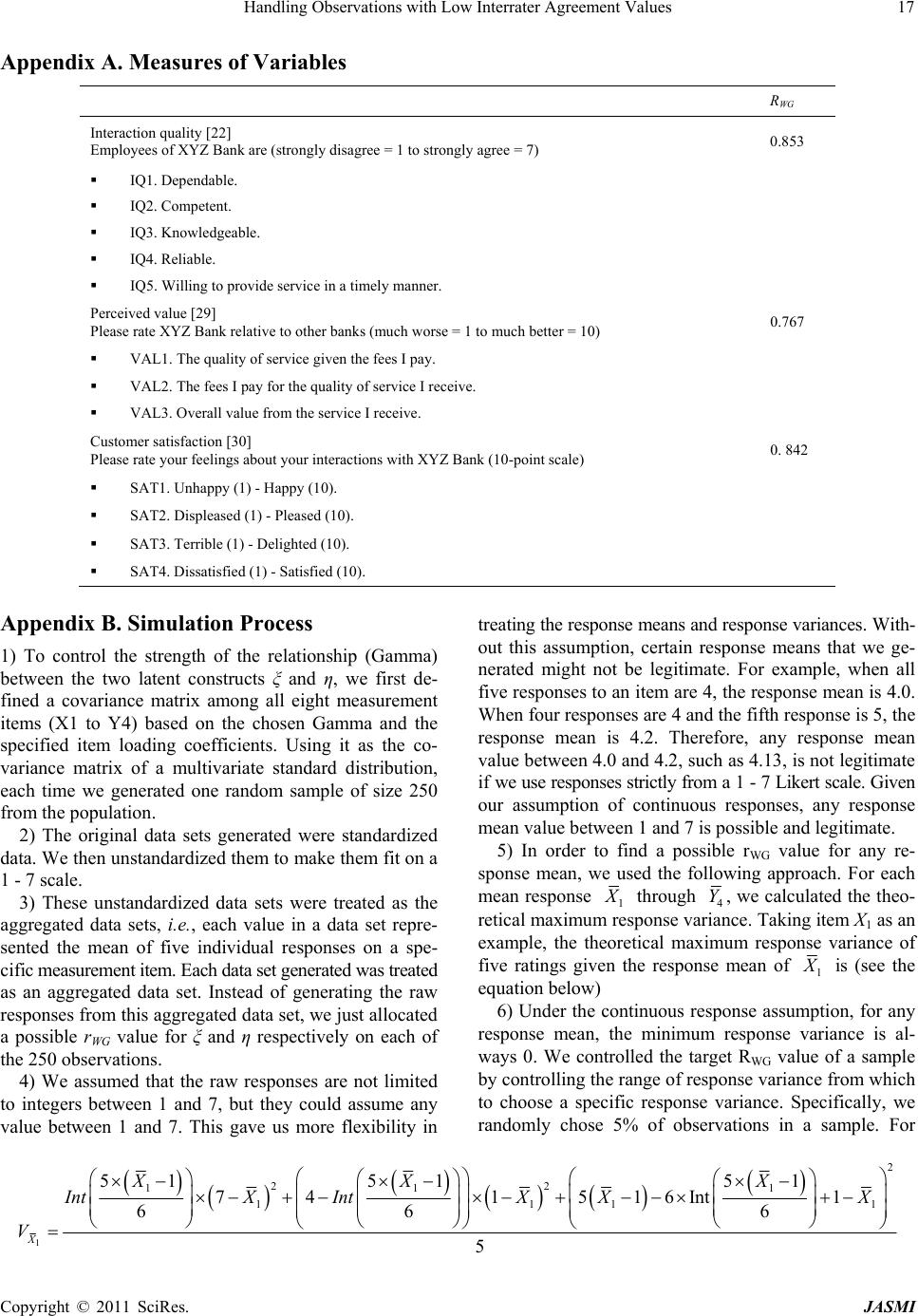

Handling Observations with Low Interrater Agreement Values17
Appendix A. Measures of Variables
RWG
Interaction quality [22]
Employees of XYZ Bank are (strongly disagree = 1 to strongly agree = 7) 0.853
 IQ1. Dependable.
 IQ2. Competent.
 IQ3. Knowledgeable.
 IQ4. Reliable.
 IQ5. Willing to provide service in a timely manner.
Perceived value [29]
Please rate XYZ Bank relative to other banks (much worse = 1 to much better = 10) 0.767
 VAL1. The quality of service given the fees I pay.
 VAL2. The fees I pay for the quality of service I receive.
 VAL3. Overall value from the service I receive.
Customer satisfaction [30]
Please rate your feelings about your interactions with XYZ Bank (10-point scale) 0. 842
 SAT1. Unhappy (1) - Happy (10).
 SAT2. Displeased (1) - Pleased (10).
 SAT3. Terrible (1) - Delighted (10).
 SAT4. Dissatisfied (1) - Satisfied (10).
Appendix B. Simulation Process
1) To control the strength of the relationship (Gamma)
between the two latent constructs ξ and η, we first de-
fined a covariance matrix among all eight measurement
items (X1 to Y4) based on the chosen Gamma and the
specified item loading coefficients. Using it as the co-
variance matrix of a multivariate standard distribution,
each time we generated one random sample of size 250
from the population.
2) The original data sets generated were standardized
data. We then unstandardized them to make them fit on a
1 - 7 scale.
3) These unstandardized data sets were treated as the
aggregated data sets, i.e., each value in a data set repre-
sented the mean of five individual responses on a spe-
cific measurement item. Each data set generated was treated
as an aggregated data set. Instead of generating the raw
responses from this aggregated data set, we just allocated
a possible rWG value for ξ and η respectively on each of
the 250 observations.
4) We assumed that the raw responses are not limited
to integers between 1 and 7, but they could assume any
value between 1 and 7. This gave us more flexibility in
treating the response means and response variances. With-
out this assumption, certain response means that we ge-
nerated might not be legitimate. For example, when all
five responses to an item are 4, the response mean is 4.0.
When four responses are 4 and the fifth response is 5, the
response mean is 4.2. Therefore, any response mean
value between 4.0 and 4.2, such as 4.13, is not legitimate
if we use responses strictly from a 1 - 7 Likert scale. Given
our assumption of continuous responses, any response
mean value between 1 and 7 is possible and legitimate.
5) In order to find a possible rWG value for any re-
sponse mean, we used the following approach. For each
mean response 1
X
through 4 Y, we calculated the theo-
retical maximum response variance. Taking item X1 as an
example, the theoretical maximum response variance of
five ratings given the response mean of 1
X
is (see the
equation below)
6) Under the continuous response assumption, for any
response mean, the minimum response variance is al-
ways 0. We controlled the target RWG value of a sample
by controlling the range of response variance from which
to choose a specific response variance. Specifically, we
randomly chose 5% of observations in a sample. For

   
1
2
22
11 1
111
51 5151
741516Int 1
66 6
5
X
XX X
IntXIntX XX
V

 
 

 
  
 

 


1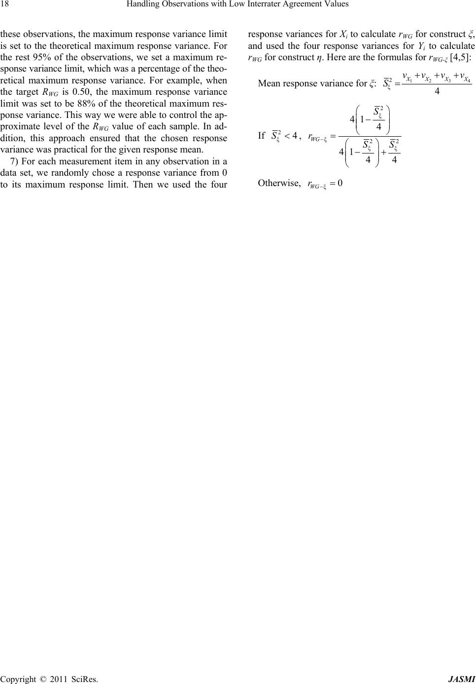





Handling Observations with Low Interrater Agreement Values
18
these observations, the maximum response variance limit
is set to the theoretical maximum response variance. For
the rest 95% of the observations, we set a maximum re-
sponse variance limit, which was a percentage of the theo-
retical maximum response variance. For example, when
the target RWG is 0.50, the maximum response variance
limit was set to be 88% of the theoretical maximum res-
ponse variance. This way we were able to control the ap-
proximate level of the RWG value of each sample. In ad-
dition, this approach ensured that the chosen response
variance was practical for the given response mean.
7) For each measurement item in any observation in a
data set, we randomly chose a response variance from 0
to its maximum response limit. Then we used the four
response variances for Xi to calculate rWG for construct ξ,
and used the four response variances for Yi to calculate
rWG for construct η. Here are the formulas for rWG-ξ [4,5]:
Mean response variance for ξ: 123
2
ξ4
XX XX
vvvv
S 4
If ,
2
ξ
ξ22
ξξ
41 4
41 44
WG
S
rSS











2
ξ4S

Otherwise, ξ0
WG
r
