Journal of Quantum Informatio n Science, 2011, 1, 127-134
doi:10.4236/jqis.2011.13018 Published Online December 2011 (http://www.SciRP.org/journal/jqis)
127
Quantitative Determination of Material Hardnes s
Zdzislaw Pluta, Tadeusz Hryniewicz
Politechnika Koszalinska, Koszalin, Poland
Received July 12, 2011; revised August 16, 2011; accepted August 22, 2011
Abstract
The paper contains description of a new quantitative method of evaluation of material hardness. First the es-
sence of cognition subject, concerned with the hardness notion, has been discussed. Next some characteris-
tics of exemplary existing evaluation methods have been presented. Then the attention was paid to the mis-
takes present in understanding/reasoning of the discussed problem. The revolutionary new method is given in
the next part of the paper by presenting functional and parametric characteristics of the process of local de-
formation of a material. At the end, the justification—with the essential meaning for investigations of present
and newer materials—to introduce one unified quantitative method of hardness evaluation, has been deliv-
ered.
Keywords: Hardness, Meyer’s Law, Hardness Modulus, Young’s Modulus, Path Constant
1. Introduction
The problem of quantitative evaluation of solid (material)
hardness is so vast/extensive that presentation of the
whole existent knowledge would require several elabora-
tions. At the same time, there are new methods proposed,
by leaving apart some others, on how to determine and/
or improve them. It seems to be no need to analyze all
the methods though some of them should be taken into
consideration to present “the development” of the prob-
lem. First of all we should take apart the formation of
newer and other methods leading to differentiation of the
results.
There is lack of synthesis, with the new scientific ac-
tions going rather forward, without primary description
of the natural reality. One should adequately quantita-
tively describe the phenomenon of local deformations of
a material that is the essence of its hardness. Therefore
let us return to the source! The development does not
rely on uncritical acceptance of existent knowledge and
continuous producing of new technical solutions. In the
analysis, any erroneous well grounded principles or laws
should be removed.
There is a law which does not reflect the reality in de-
termination of material’s hardness and that is the Meyer’s
law which will be presented here. Also some other rules,
described using a function of the same class, which de-
form the reality should be removed.
A critical approach to the existent reality should pre-
vail. In the paper, first the essence of hardness notion
will be analyzed. Then the characteristics of exemplary
methods of quantitative evaluation of material hardness
will be given. After that, the erroneous reasoning will be
presented. Afterwards the new method of determination
of material hardness will be given. Functional and para-
metric characteristics of the process of local material
deformation, being physical and measurable/determin-
able magnitude, will be presented.
Let us present the notion of hardness and indicate dif-
ferent understanding of this magnitude. For defining the
hardness, the dictionary [1] includes definition of rigidity
as “lack of rigidity, elasticity” and it is rather pseudode-
finition. Furthermore, the same source [1] defines the
hardness as “the magnitude of deformation occurred un-
der action of concentrated forces (acting on a small area
of the studied material)”. There also, one of the measures
of hardness is given, without an explanation of this no-
tion. Some sources [2,3] simply say that “the hardness of
a material measures how tightly the atoms are held to-
gether within it” [2] or describe more extensively that
“hardness is not an intrinsic property of any material,
(like density or melting point), it is rather a characteristic
deriving from the composition, the thermal and me-
chanical history of the material, and essentially from the
structure (or more properly the microstructure) of the
specimen involved” [3].
In [4] the following definition of hardness is given:
“Hardness is the resistance of a material to a firm defor-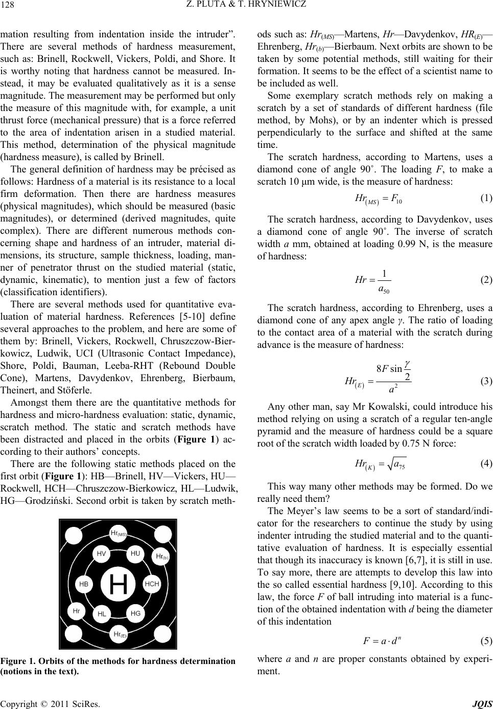

128 Z. PLUTA & T. HRYNIEWICZ
mation resulting from indentation inside the intruder”.
There are several methods of hardness measurement,
such as: Brinell, Rockwell, Vickers, Poldi, and Shore. It
is worthy noting that hardness cannot be measured. In-
stead, it may be evaluated qualitatively as it is a sense
magnitude. The measurement may be performed but only
the measure of this magnitude with, for example, a unit
thrust force (mechanical pressure) that is a force referred
to the area of indentation arisen in a studied material.
This method, determination of the physical magnitude
(hardness measure), is called by Brinell.
The general definition of hardness may be précised as
follows: Hardness of a material is its resistance to a local
firm deformation. Then there are hardness measures
(physical magnitudes), which should be measured (basic
magnitudes), or determined (derived magnitudes, quite
complex). There are different numerous methods con-
cerning shape and hardness of an intruder, material di-
mensions, its structure, sample thickness, loading, man-
ner of penetrator thrust on the studied material (static,
dynamic, kinematic), to mention just a few of factors
(classification identifiers).
There are several methods used for quantitative eva-
luation of material hardness. References [5-10] define
several approaches to the problem, and here are some of
them by: Brinell, Vickers, Rockwell, Chruszczow-Bier-
kowicz, Ludwik, UCI (Ultrasonic Contact Impedance),
Shore, Poldi, Bauman, Leeba-RHT (Rebound Double
Cone), Martens, Davydenkov, Ehrenberg, Bierbaum,
Theinert, and Stöferle.
Amongst them there are the quantitative methods for
hardness and micro-hardness evaluation: static, dynamic,
scratch method. The static and scratch methods have
been distracted and placed in the orbits (Figure 1) ac-
cording to their authors’ concepts.
There are the following static methods placed on the
first orbit (Figure 1): HB—Brinell, HV—Vickers, HU—
Rockwell, HCH—Chruszczow-Bierkowicz, HL—Ludwik,
HG—Grodziński. Second orbit is taken by scratch meth-
Figure 1. Orbits of the methods for hardness determination
(notions in the text).
ods such as: Hr(MS)—Martens, Hr—Davydenkov, HR(E)—
Ehrenberg, Hr(b)—Bierbaum. Next orbits are shown to be
taken by some potential methods, still waiting for their
formation. It seems to be the effect of a scientist name to
be included as well.
Some exemplary scratch methods rely on making a
scratch by a set of standards of different hardness (file
method, by Mohs), or by an indenter which is pressed
perpendicularly to the surface and shifted at the same
time.
The scratch hardness, according to Martens, uses a
diamond cone of angle 90˚. The loading F, to make a
scratch 10 μm wide, is the measure of hardness:

10 MS
H
rF (1)
The scratch hardness, according to Davydenkov, uses
a diamond cone of angle 90˚. The inverse of scratch
width a mm, obtained at loading 0.99 N, is the measure
of hardness:
50
1
Hr a  (2)
The scratch hardness, according to Ehrenberg, uses a
diamond cone of any apex angle γ. The ratio of loading
to the contact area of a material with the scratch during
advance is the measure of hardness:
 2
8sin
2
E
F
Hr a

 (3)
Any other man, say Mr Kowalski, could introduce his
method relying on using a scratch of a regular ten-angle
pyramid and the measure of hardness could be a square
root of the scratch width loaded by 0.75 N force:

75 K
H
ra (4)
This way many other methods may be formed. Do we
really need them?
The Meyer’s law seems to be a sort of standard/indi-
cator for the researchers to continue the study by using
indenter intruding the studied material and to the quanti-
tative evaluation of hardness. It is especially essential
that though its inaccuracy is known [6,7], it is still in use.
To say more, there are attempts to develop this law into
the so called essential hardness [9,10]. According to this
law, the force F of ball intruding into material is a func-
tion of the obtained indentation with d being the diameter
of this indentation
n
F
ad (5)
where a and n are proper constants obtained by experi-
ment.
C
opyright © 2011 SciRes. JQIS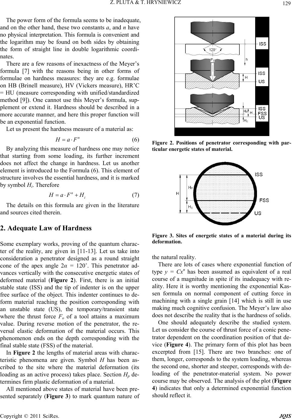

129 Z. PLUTA & T. HRYNIEWICZ
The power form of the formula seems to be inadequate,
and on the other hand, these two constants a, and n have
no physical interpretation. This formula is convenient and
the logarithm may be found on both sides by obtaining
the form of straight line in double logarithmic coordi-
nates.
There are a few reasons of inexactness of the Meyer’s
formula [7] with the reasons being in other forms of
formulae on hardness measures: they are e.g. formulae
on HB (Brinell measure), HV (Vickers measure), HR’C
= HU (measure corresponding with unified/standardized
method [9]). One cannot use this Meyer’s formula, sup-
plement or extend it. Hardness should be described in a
more accurate manner, and here this proper function will
be an exponential function.
Let us present the hardness measure of a material as:
n
H
aF (6)
By analyzing this measure of hardness one may notice
that starting from some loading, its further increment
does not affect the change in hardness. Let us another
element is introduced to the Formula (6). This element of
structure involves the essential hardness, and it is marked
by symbol Hi. Therefore
n
i
H
aF H (7)
The details on this formula are given in the literature
and sources cited therein.
2. Adequate Law of Hardness
Some exemplary works, proving of the quantum charac-
ter of the reality, are given in [11-13]. Let us take into
consideration a penetrator designed as a round straight
cone of the apex angle 2α = 120˚. This penetrator ad-
vances vertically with the consecutive energetic states of
deformed material (Figure 2). First, there is an initial
stable state (ISS) and the tip of indenter is on the upper
free surface of the object. This indenter continues to de-
form material reaching the position corresponding with
an unstable state (US), the temporary/transient state
where the thrust force Fo of a tool attains a maximum
value. During reverse motion of the penetrator, the re-
versal elastic deformation of the material occurs. This
phenomenon ends on the depth corresponding with the
final stable state (FSS) of the material.
In Figure 2 the lengths of material areas with charac-
teristic phenomena are given. Symbol H has been as-
cribed to the site where the material deformation (its
loading as an active process) takes place. Section Hp de-
termines firm plastic deformation of a material.
All mentioned above states of material have been pre-
sented separately (Figure 3) to mark quantum nature of
Figure 2. Positions of penetrator corresponding with par-
ticular energetic states of material.
Figure 3. Sites of energetic states of a material during its
deformation.
the natural reality.
There are lots of cases where exponential function of
type y = Cxn has been assumed as equivalent of a real
course of a magnitude in spite if its inadequacy with re-
ality. Here it is worthy mentioning the exponential Kas-
sen formula on normal component of cutting force in
machining with a single grain [14] which is still in use
making much cognitive confusion. The Meyer’s law also
does not describe the reality that is the hardness of solids.
One should adequately describe the studied system.
Let us consider the course of thrust force of a conic pene-
trator dependent on the coordination position of that de-
vice (Figure 4). The primary form of this plot has been
excerpted from [15]. There are two branches: one of
them, longer, corresponds to the system loading, whereas
the second one, shorter and steeper, corresponds with de-
loading of the penetrator-material system. No power
course may be observed. The analysis of the plot (Figure
4) indicates that only a determined exponential function
hould reflect it. s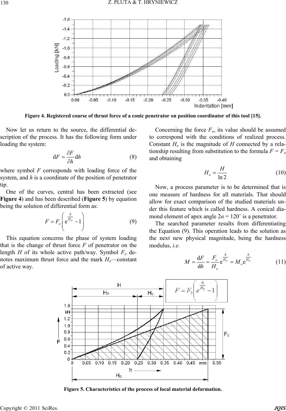

Z. PLUTA & T. HRYNIEWICZ
130
Figure 4. Registered course of thrust force of a conic penetrator on position coordinator of this tool [15].
Concerning the force Fo, its value should be assumed
to correspond with the conditions of realized process.
Constant Ho is the magnitude of H connected by a rela-
tionship resulting from substitution to the formula F = Fo
and obtaining
Now let us return to the source, the differential de-
scription of the process. It has the following form under
loading the system:
d
Fd
F
h
h

 (8)
ln 2
o
H
H (10)
where symbol F corresponds with loading force of the
system, and h is a coordinate of the position of penetrator
tip. Now, a process parameter is to be determined that is
one measure of hardness for all materials. That should
allow for exact comparison of the studied materials un-
der this feature which is called hardness. A conical dia-
mond element of apex angle 2α = 120˚ is a penetrator.
One of the curves, central has been extracted (see
Figure 4) and has been described (Figure 5) by equation
being the solution of differential form as:
e1
o
h
H
o
FF







(9) The searched parameter results from differentiating
the Equation (9). This operation leads to the solution as
the next new physical magnitude, being the hardness
modulus, i.e.
This equation concerns the phase of system loading
that is the change of thrust force F of penetrator on the
length H of its whole active path/way. Symbol Fo de-
notes maximum thrust force and the mark Ho—constant
of active way.
de
d
o
hh
e
o
H
H o
o
o
F
F
M
hH
 M
(11)
Figure 5. Characteristics of the process of local material deformation.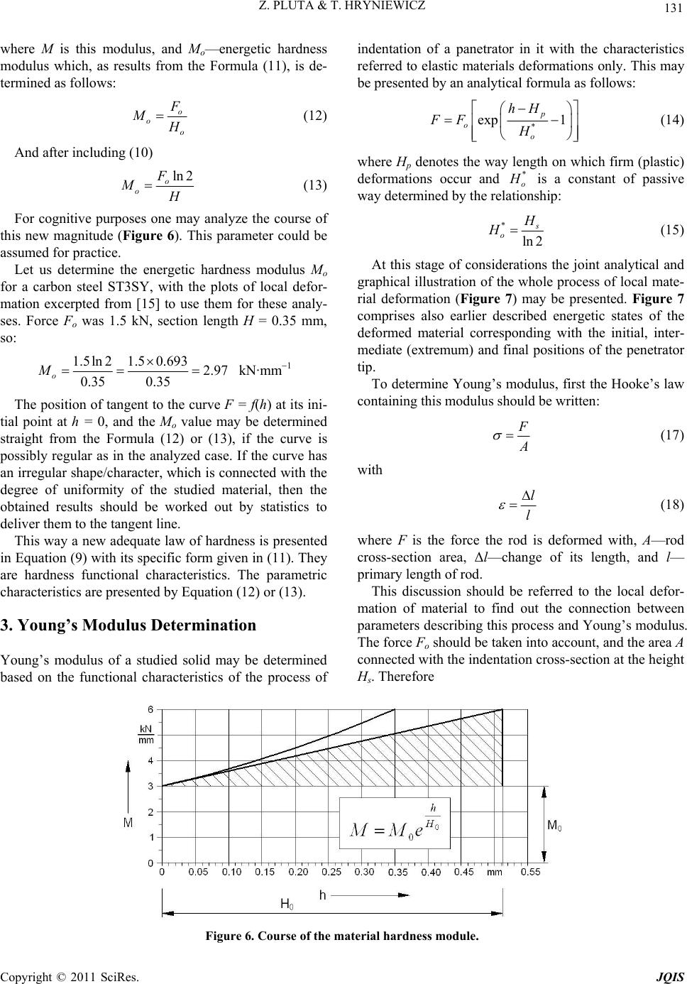

131 Z. PLUTA & T. HRYNIEWICZ
where M is this modulus, and Mo—energetic hardness
modulus which, as results from the Formula (11), is de-
termined as follows:
o
o
o
F
M
H
 (12)
And after including (10)
ln 2
o
o
F
M
H
 (13)
For cognitive purposes one may analyze the course of
this new magnitude (Figure 6). This parameter could be
assumed for practice.
Let us determine the energetic hardness modulus Mo
for a carbon steel ST3SY, with the plots of local defor-
mation excerpted from [15] to use them for these analy-
ses. Force Fo was 1.5 kN, section length H = 0.35 mm,
so:
1.5ln 21.50.6932.97
0.35 0.35
o
M   kN·mm1
The position of tangent to the curve F = f(h) at its ini-
tial point at h = 0, and the Mo value may be determined
straight from the Formula (12) or (13), if the curve is
possibly regular as in the analyzed case. If the curve has
an irregular shape/character, which is connected with the
degree of uniformity of the studied material, then the
obtained results should be worked out by statistics to
deliver them to the tangent line.
This way a new adequate law of hardness is presented
in Equation (9) with its specific form given in (11). They
are hardness functional characteristics. The parametric
characteristics are presented by Equation (12) or (13).
3. Young’s Modulus Determination
Young’s modulus of a studied solid may be determined
based on the functional characteristics of the process of
indentation of a panetrator in it with the characteristics
referred to elastic materials deformations only. This may
be presented by an analytical formula as follows:
*
exp 1
p
o
o
hH
FF H

 



 





(14)
where Hp denotes the way length on which firm (plastic)
deformations occur and *
o
H
is a constant of passive
way determined by the relationship:
*
ln 2
s
o
H
H (15)
At this stage of considerations the joint analytical and
graphical illustration of the whole process of local mate-
rial deformation (Figure 7) may be presented. Figure 7
comprises also earlier described energetic states of the
deformed material corresponding with the initial, inter-
mediate (extremum) and final positions of the penetrator
tip.
To determine Young’s modulus, first the Hooke’s law
containing this modulus should be written:
F
A


(17)
with
l
l


 (18)
where F is the force the rod is deformed with, A—rod
cross-section area, Δl—change of its length, and l—
primary length of rod.
This discussion should be referred to the local defor-
mation of material to find out the connection between
parameters describing this process and Young’s modulus.
The force Fo should be taken into account, and the area A
connected with the indentation cross-section at the height
Hs. Therefore
Figure 6. Course of the material har dness module.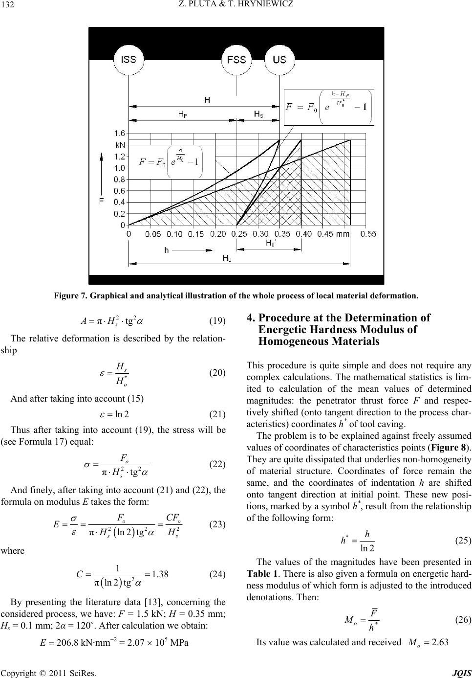

132 Z. PLUTA & T. HRYNIEWICZ
Figure 7. Graphical and analytical illustration of the whole process of local material deformation.
22
πtg
s
AH

  (19)
The relative deformation is described by the relation-
ship
*
s
o
H
H
  (20)
And after taking into account (15)
ln 2

 (21)
Thus after taking into account (19), the stress will be
(see Formula 17) equal:
22
πtg
o
s
F
H


 (22)
And finely, after taking into account (21) and (22), the
formula on modulus E takes the form:

22
πln 2tg
o
2
o
s
s
F
CF
E
H
H


 
 (23)
where

2
11.38
πln 2tg
C

 (24)
By presenting the literature data [13], concerning the
considered process, we have: F = 1.5 kN; H = 0.35 mm;
Hs = 0.1 mm; 2α = 120˚. After calculation we obtain:
206.8EkN·mm2 = 2.07  105 MPa
4. Procedure at the Determination of
Energetic Hardness Modulus of
Homogeneous Materials
This procedure is quite simple and does not require any
complex calculations. The mathematical statistics is lim-
ited to calculation of the mean values of determined
magnitudes: the penetrator thrust force F and respec-
tively shifted (onto tangent direction to the process char-
acteristics) coordinates h* of tool caving.
The problem is to be explained against freely assumed
values of coordinates of characteristics points (Figure 8).
They are quite dissipated that underlies non-homogeneity
of material structure. Coordinates of force remain the
same, and the coordinates of indentation h are shifted
onto tangent direction at initial point. These new posi-
tions, marked by a symbol h*, result from the relationship
of the following form:
*
ln 2
h
h (25)
The values of the magnitudes have been presented in
Table 1. There is also given a formula on energetic hard-
ness modulus of which form is adjusted to the introduced
denotations. Then:
*
o
F
Mh  (26)
Its value was calculated and received 2.63
o
M
C
opyright © 2011 SciRes. JQIS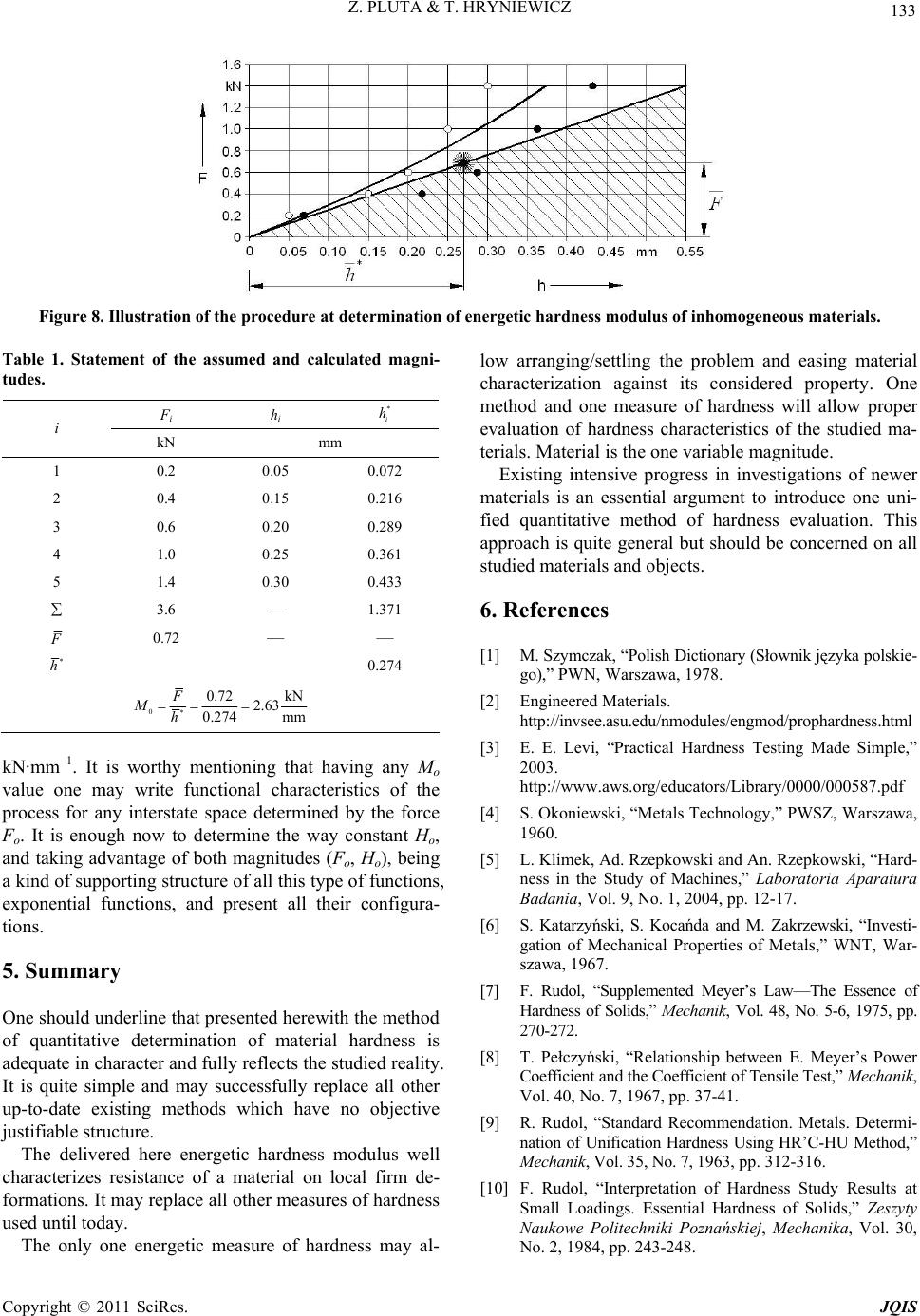

133 Z. PLUTA & T. HRYNIEWICZ
Figure 8. Illustration of the procedure at determination of energetic hardness modulus of inhomogeneous materials.
Table 1. Statement of the assumed and calculated magni-
tudes.
Fi h
i * i
h
i
kN mm
1 0.2 0.05 0.072
2 0.4 0.15 0.216
3 0.6 0.20 0.289
4 1.0 0.25 0.361
5 1.4 0.30 0.433
 3.6 — 1.371
F
0.72 — —
*
h 0.274
0*
0.72 kN
2.63
0.274 mm
F
Mh  
kN·mm1. It is worthy mentioning that having any Mo
value one may write functional characteristics of the
process for any interstate space determined by the force
Fo. It is enough now to determine the way constant Ho,
and taking advantage of both magnitudes (Fo, Ho), being
a kind of supporting structure of all this type of functions,
exponential functions, and present all their configura-
tions.
5. Summary
One should underline that presented herewith the method
of quantitative determination of material hardness is
adequate in character and fully reflects the studied reality.
It is quite simple and may successfully replace all other
up-to-date existing methods which have no objective
justifiable structure.
The delivered here energetic hardness modulus well
characterizes resistance of a material on local firm de-
formations. It may replace all other measures of hardness
used until today.
The only one energetic measure of hardness may al-
low arranging/settling the problem and easing material
characterization against its considered property. One
method and one measure of hardness will allow proper
evaluation of hardness characteristics of the studied ma-
terials. Material is the one variable magnitude.
Existing intensive progress in investigations of newer
materials is an essential argument to introduce one uni-
fied quantitative method of hardness evaluation. This
approach is quite general but should be concerned on all
studied materials and objects.
6. References
[1] M. Szymczak, “Polish Dictionary (Słownik języka polskie-
go),” PWN, Warszawa, 1978.
[2] Engineered Materials.
http://invsee.asu.edu/nmodules/engmod/prophardness.html
[3] E. E. Levi, “Practical Hardness Testing Made Simple,”
2003.
http://www.aws.org/educators/Library/0000/000587.pdf
[4] S. Okoniewski, “Metals Technology,” PWSZ, Warszawa,
1960.
[5] L. Klimek, Ad. Rzepkowski and An. Rzepkowski, “Hard-
ness in the Study of Machines,” Laboratoria Aparatura
Badania, Vol. 9, No. 1, 2004, pp. 12-17.
[6] S. Katarzyński, S. Kocańda and M. Zakrzewski, “Investi-
gation of Mechanical Properties of Metals,” WNT, War-
szawa, 1967.
[7] F. Rudol, “Supplemented Meyer’s Law—The Essence of
Hardness of Solids,” Mechanik, Vol. 48, No. 5-6, 1975, pp.
270-272.
[8] T. Pełczyński, “Relationship between E. Meyer’s Power
Coefficient and the Coefficient of Tensile Test,” Mechanik,
Vol. 40, No. 7, 1967, pp. 37-41.
[9] R. Rudol, “Standard Recommendation. Metals. Determi-
nation of Unification Hardness Using HR’C-HU Method,”
Mechanik, Vol. 35, No. 7, 1963, pp. 312-316.
[10] F. Rudol, “Interpretation of Hardness Study Results at
Small Loadings. Essential Hardness of Solids,” Zeszyty
Naukowe Politechniki Poznańskiej, Mechanika, Vol. 30,
No. 2, 1984, pp. 243-248.

134 Z. PLUTA & T. HRYNIEWICZ
[11] Z. Pluta, “On the Oblique Flight of a Body across the
Gravitation Space-Times,” Nauka Innowacje Technika,
Vol. 7-8, No. 5-6, 2004, pp. 58-61.
[12] Z. Pluta, “Of the d’Alembert’s Rule with the Contents
Permeated by Fiction and ... a Phantasy,” Laboratoria
Aparatura Badania, Vol. 9, No. 6, 2004, pp. 42-46.
[13] Z. Pluta, “On the R-F Scientific Chain,” Koszalinskie Stu-
dia i Materiały, Vol. 7, No. 1, 2004, pp. 131-143.
[14] G. Kassen, “Beschreibung der Elementaren Kinematik
Les Schleifvorganges,” Ph.D. Dissertation, RWTH Aa-
chen University, Aachen, 1969.
[15] J. Bochnia, “Young’s Modulus Determination Based on
Statistic Test of the Cone Indentation,” Archiwum Tech-
nologii Maszyn i Automatyzacji, Vol. 22, No. 2, 2002, pp.
41-48.
C
opyright © 2011 SciRes. JQIS