American Journal of Computational Mathematics, 2011, 1, 318-327
doi:10.4236/ajcm.2011.14038 Published Online December 2011 (http://www.SciRP.org/journal/ajcm)
A New Fourth Order Difference Approximation for the
Solution of Three-Dimensional Non-Linear Biharmonic
Equations Using Coupled Approach
Ranjan Kumar Mohanty1, Mahinder Kumar Jain2*, Biranchi Narayan Mishra3#
1Department of Mat hem at i cs, Faculty of Mathematical Sciences, University of Delhi, Delhi, India
2Department of Mat hem at i cs, Indian Institute of Technology, New Delhi, Indi a
3Department of Mat hem at i cs, Utkal University, Bhubaneswar, India
Received October 13, 2011; revised November 2, 2011; accepted November 9, 2011
Abstract
This paper deals with a new higher order compact difference scheme, which is, O(h4) using coupled ap-
proach on the 19-point 3D stencil for the solution of three dimensional nonlinear biharmonic equations. At
each internal grid point, the solution u(x, y, z) and its Laplacian 2u

are obtained. The resulting stencil al-
gorithm is presented and hence this new algorithm can be easily incorporated to solve many problems. The
present discretization allows us to use the Dirichlet boundary conditions only and there is no need to discre-
tize the derivative boundary conditions near the boundary. We also show that special treatment is required to
handle the boundary conditions. Convergence analysis for a model problem is briefly discussed. The method
is tested on three problems and compares very favourably with the corresponding second order approxima-
tion which we also discuss using coupled approach.
Keywords: Three-Dimensional Non-Linear Biharmonic Equation, Finite Differences, Fourth Order Accuracy,
Compact Discretization, Block-Block-Tridiagonal, Tangential Derivatives, Laplacian, Stream
Function, Reynolds Number
1. Introduction
We are interested to develop a new algorithm for solving
the three-dimensional non-linear biharmonic partial dif-
ferential equation


444
4
444
444
2222 22
22 22
,,
2
,,,, ,,,,,,
0,,1

x
yzx y z
uuu
uxyz xyz
uuu
xy yz zx
f
xyzuu uuuuuu
xyx







 




(1)
defined in the solution region
 
,, 0,,1xyz xyz with boundary , where


222
2
22
,, uu uxyz
mensional Laplacians of u in . We assume that the
solution u(x, y, z) is smooth enough to maintain the order
and accuracy of the algorithm as high as possible under
consideration.

The Dirichlet boundary conditions are given by
 
2
12
2
,, ,,, , ,,
u
ufxyzfxyz xyz
n



. (2)
The nonlinear biharmonic equation is a fourth order
elliptic partial differential equation which occurs in many
areas of physics and applied mathematics, especially in
elasticity theory and stokes flow problems. It occurs with
fluid flowing over an obstacle or with the movement of a
natural or artificial body. Common examples are the
flows past an airplane, a submarine, an automobile, or
wind blowing past a high-rise building. Till about three
and half decades ago, second order accuracy was consid-
ered to be sufficient for most biharmonic problems. In
particular, the central difference schemes have been the
most popular ones because of their straightforwardness
2
u
x
yz



represents the three di-
*Present address: 4076, C/4, Vasant Kunj, New Delhi, India.
#Present address: Department of Mathematics, Rajasunakhala College,
N
ayagarh, Orissa, India.

R. K. MOHANTY ET AL.319
in application. Though for problems having well behaved
solutions, the solution may be of poor quality for con-
vection dominated flows, or for high Reynolds number if
the mesh is not sufficiently refined. Again, higher order
discretization is generally associated with non-compact
stencil which increase the band-width of the resultant
coefficient matrix. Both mesh refinement and increased
matrix band-width invariably lead to a large number of
arithmetic operations. Thus neither a lower order accu-
rate method on a fine mesh nor a higher order accurate
one on a non-compact stencil seems to be computation-
ally cost-effective. This is where higher order compact
(HOC) finite difference methods become important. A
compact finite difference schemes is one which utilizes
grid points located only directly adjacent to the node
about which differences are taken. In addition, if the
scheme has an accuracy greater than two, it is termed as
HOC method. The higher order accuracy of the HOC
methods combined with the compactness of the differ-
ence stencils yields highly accurate numerical solutions
on relatively coarser grids with greater computational
efficiency. A compact difference scheme is one that is
restricted to the patch of cells immediately surrounding
any given node and does not extend further. Most stan-
dard difference schemes such as the central difference
scheme for second order elliptic partial differential equa-
tions are compact. The high order compact method con-
sidered here is different in that the governing differential
equation is used to approximate the lower order deriva-
tive terms with the imbedding technique. The scheme is
difficult to develop due to the need for extensive alge-
braic manipulation, especially for non-linear problems.
However, once high-order method developed, it can be
incorporated easily in application. Various approaches
for the numerical solution of 2D biharmonic problems
has been discussed in the literature. Not many authors
have tried to solve the three-dimensional biharmonic
problems. The reason is that for high order approxima-
tion it is difficult to discretize the nonlinear biharmonic
equation as well as the associated boundary conditions
using a single computational cell. Another reason of ne-
cessity is that three-dimensional problems require large
computing power and place huge amount of memory
requirements on the computational systems. Such com-
puting power has only recently begun to become avail-
able for academic research. Smith [1] and Ehrlich [2,3]
have used coupled approach and solved 2D biharmonic
equation using second order accurate finite difference
equations. Bauer and Riess [4] have used block iterative
method to solve block 5-diagonal matrices for the solu-
tion of 2D biharmonic problem of first kind. Glowinski
and Pironneau [5] have developed a stable lower order
numerical method for the first biharmonic problem. Later,
kwon et al. [6], Stephenson [7], and Mohanty et al. [8-12]
have developed certain second- and fourth-order finite
difference methods for the solution of two and three di-
mensional biharmonic problems using single compact
cells. Recently, using more grid points Singh et al [13]
and Khattar et al. [14] have discussed the fourth order
numerical methods for the solution of 2D and 3D bihar-
monic problems of second kind. Further, using coupled
approach Mohanty [15] has derived a new nine point
fourth order finite difference method for the solution of
non-linear biharmonic problems of second kind. In most
recently, using nine point compact cell Mohanty et al. [16]
have discussed fourth order finite difference method for
the solution of nonlinear 2D triharmonic problems. Ear-
lier, Mohanty et al. [17-19] have developed fourth order
compact difference schemes for the solution of multi-
dimensional non-linear elliptic partial differential equa-
tions. Fourth order compact difference schemes have
become quite popular as against the other lower order
accurate schemes which require high mesh refinement
and hence are computationally inefficient. On the other
hand, the higher order accuracy of the fourth order com-
pact methods combined with the compactness of the dif-
ference stencil yields highly accurate numerical solutions
on relatively coarser grids with greater computational
efficiency. A conventional approach for solving the 3D
biharmonic equation is to discretize the differential Equa-
tion (1) on a uniform grid using 125-point approxima-
tions with truncation error of order . This approxima-
tion connect the values of central point in terms of 124
neighbouring values of u in 55 cubic grid. We
note that the central value of u is connected to grid points
two grids away in each direction from the central point
and the difference approximations needs to be modified
at grid points near the boundaries. There are serious
computational difficulties with solution of the linear and
non-linear systems obtained through 125-point discreti-
zation of the 3D biharmonic equation. Approximations
using compact cells avoid these difficulties. The compact
approach involves discretizing the biharmonic equations
using not just the grid values of the unknown solution u
but also the values of the derivatives
2
h
5 
x
x, u
y
y and u
z
z
at selected grid points (see Mohanty and Pandey [10]). It
is required to solve the system of four equations to obtain
the solutions of
u
,
x
x
uu,
y
y and u
z
z
u. In this paper, we
write the original differential equation in a coupled man-
ner and introduce new concepts to handle the boundary
conditions without discretizing them. For fourth order
approximations we use only 19-point compact cell (see
Figure 1). No approximations for derivatives need to be
carried out at the boundaries and the given Dirichlet
boundary conditions are exactly satisfied. The main ad-
vantage of this work is that we require to solve a system
of two equations, whereas in our previous work [10], we
were required to solve a system of four equations to ob-

R. K. MOHANTY ET AL. 320
(
x
l
, y
m+1
,
z
n+1
)
(x
l+1
, y
m
, z
n+1
) (x
l-1
, y
m
, z
n+1
)
(x
l-1
, y
m
, z
n-1
) (x
l+1
, y
m
, z
n-1
)
(x
l
, y
m-1
, z
n-1
)
(x
l+1
, y
m+1
, z
n
)
(x
l-1
, y
m+1
, z
n
)
(x
l
, y
m-1
, z
n+1
)
(x
l-1
, y
m
, z
n
)
(x
l-1
, y
m-1
, z
n
) (x
l+1
, y
m-1
, z
n
)
(x
l
, y
m
, z
n-1
)
(x
l
, y
m+1
, z
n-1
)
(x
l
, y
m
, z
n
)
(x
l
, y
m
, z
n+1
)
(x
l
, y
m-1
, z
n
)
(x
l+1
, y
m
, z
n
)
(x
l
, y
m+1
, z
n
)
Figure 1. 19-point 3D single computational cell.
tain the numerical solution of u(x, y, z). Thus the pro-
posed method requires less algebraic operations as com-
pared to the method discussed in [10]. In Section 2, we
give the formulation of the method. The complete deri-
vation of the method is carried out in Section 3. In order
to validate the proposed fourth order method and test its
robustness, we solve three problems in Section 4 and
also discussed stability analysis briefly for a model pro-
blem. Concluding remarks are presented in Section 5.
2. Formulation of the Fourth Order
Discretization
Consider the three-dimensional solution region

,
which is replaced by a set of grid points (xl, ym, zn),
where h > 0 is the mesh sizes in x-, y- and z- directions,
and grid points are defined by xl = lh, ym = mh, zn = nh; l,
m, n = 0 (1) N + 1 with (N + 1) h = 1. Let ,,lmn and
,,lmn be the approximate and exact solution values of
u(x, y, z) at the grid point (xl, ym, zn ), respectively.
u
U
The Dirichlet boundary conditions are given by (2).
Since the grid lines are parallel to coordinate axes and
the values of u are exactly known on the boundary, this
implies, the successive tangential partial derivatives of u
are known exactly on the boundary. For example, on the
plane y = 0, the values of u(x, 0, z) and are
known, i.e., the values of x ux , ,
, ,··· etc are known on the plane
(,0,)
yy
uxz
,)z(,0
z
ux(,0 ,)z
(,0,)
xx
ux z(,0,)
zz
ux z
y = 0. This implies, the values of u(x, 0, z) and



2, 0,, 0,, 0,,0,
xx yy zz
ux zux z uxz ux z  
2u


are
known on the plane y=0. Similarly the values of u and
are known on all plane sides of the cubic region
.
Let us denote . Then we re-
formulate the boundary value problems (1) and (2) in a
coupled manner as
2(, ,)(, ,)uxyz vxyz
 

222
2
222
,,,, ,
,,
uuu
uxyz vxyz
xyz
xyz




, (3a)



222
2
222
,,
,,,,,, ,,, ,,
,,
xxyyzz
vvv
vxyz xyz
f
xyzuvu v uvu v
xyz






. (3b)
subject to the Dirichlet boundary conditions prescribed
by



 
,, ,,, ,,,uaxyzv cxyzxyz


. (4)
Let at the grid points (xl, ym, zn), the approximate and
exact solution values of v(x, y, z) be denoted as
and , respectively.
,,lmn
v
,,lmn
In order to obtain fourth order approximations on the
19-point compact cell for the system of non-linear dif-
ferential Equations (3a) and (3b), we need the following
approximations:
V

,, 1, ,1, ,
1
2
xlm nlmn lmn
UUU
h

, (5a)

,, 1, ,1, ,
1
2
xl m nlmn lmn
VVV
h


, (5b)


,, ,1, ,1,
1
2
yl m nlm nlm n
UUU
h

, (6a)

,, ,1, ,1,
1
2
ylm nlm nlm n
VVV
h


, (6b)

,, ,, 1,, 1
1
2
zl m nlmn lmn
UUU
h


, (7a)

R. K. MOHANTY ET AL.321

,, ,, 1,, 1
1
2
zl m nlmn lmn
VVV
h



, (7b)

1, ,1, ,, ,1, ,
134
2
xlm nlmnlmn lmn
UUUU
h

 

, (8a)

1, ,1, ,,,1, ,
134
2
xlm nlmnlmn lmn
VVVV
h

 

, (8b)

,1, 1, 1,1, 1,
1
2
xl mnlmnlmn
UUU
h
 
, (9a)

,1,1, 1,1, 1,
1
2
xl mnlmnlmn
VVV
h

, (9b)

,, 11,,11, ,1
1
2
xlm nlmn lmn
UUU
h
 
, (10a)

,, 11,,11, ,1
1
2
xlm nlmn lmn
VVV
h
 
, (10b)
 1, ,1,1,1, 1,
1
2
ylm nlmnlmn
UUU
h
 
, (11a)

1, ,1, 1,1, 1,
1
2
ylm nlmnlmn
VVV
h
 
, (11b)

,1, ,1,,, ,1,
134
2
yl mnlm nlmnlmn
UUUU
h

 

, (12a)

,1, ,1,,, ,1,
134
2
yl mnlm nlmnlm n
VVVV
h

 

, (12b)

,, 1,1,1 ,1,1
1
2
yl m nlmnlm n
UUU
h
 
, (13a)

,, 1,1,1 ,1,1
1
2
ylm nlm nlm n
VVV
h
 


, (13b)

1, ,1,,11, ,1
1
2
zlm nlmnlmn
UUU
h

, (14a)

1, ,1, ,11, ,1
1
2
zlm nlmnlmn
VVV
h
 


, (14b)

,1, ,1,1,1,1
1
2
zl mnlmnlm n
UUU
h
 
, (15a)

,1,,1,1 ,1,1
1
2
zl mnlmnlm n
VVV
h
 


, (15b)

,, 1,, 1,,,, 1
134
2
zlmnlmnlmn lmn
UUUU
h

  , (16a)

,, 1,, 1,,,, 1
134
2
zl m nlmnlmn lmn
VVVV
h

  , (16b)

,1, 1,1,,1,1,1,
2
12
xxl mnlmnlmn lmn
UUUU
h
 
, (17a)

,1, 1, 1,, 1,1, 1,
2
12
xxl mnlmnlmnlmn
VVVV
h
 
, (17b)

,, 11,, 1,, 11,, 1
2
12
xxl m nlmnlmn lmn
UUUU
h
 
, (18a)

,, 11,, 1,, 11,, 1
2
12
xxl m nlmnlmn lmn
VVVV
h
 
, (18b)
 1, ,1,1,1, ,1,1,
2
12
yylm nlmnlmn lmn
UUUU
h
 
, (19a)

1, ,1,1,1,,1,1,
2
12
yylm nlmnlmn lmn
VVVV
h
 
, (19b)
 ,, 1,1,1,,1 ,1,1
2
12
yylm nlm nlmnlm n
UUUU
h
 
, (20a)

,, 1,1,1,,1 ,1,1
2
12
yylm nlm nlmnlm n
VVVV
h
 
, (20b)

1, ,1,,11, ,1,,1
2
12
zzlm nlmnlmn lmn
UUUU
h
 
, (21a)

1, ,1, ,11,,1, ,1
2
12
zzlm nlmnlmnlmn
VVVV
h
 
, (21b)

,1,,1,1,1, ,1,1
2
12
zzl mnlm nlm nlm n
UUUU
h
  
, (22a)

,1, ,1,1,1, ,1,1
2
12
zzl mnlm nlm nlmn
VVVV
h
  
. (22b)
Then we need to evaluate

1, ,1, ,1, ,1, ,1, ,1, ,1, ,
11,,1,,
,,,, ,,,,,,
lmn
x
lmn xlmnylmnylmnzlmn zlmn
lmnlmnlmn
FfxyzUVUVUVUV
 

 (23)

,1,,1, ,1,,1,,1,,1, ,1,
1,1,,1,
,,,, ,,,,,, lm n
x
lm nxlmnylm nylm nzlm nzlmn
lmnlmnlmn
FfxyzUVUVUVUV  

 (24)

,, 1,,1,,1,,1,, 1,, 1,, 1
1,,1,,1
,, ,,,,,,,,
lmn xlmn xlmnylmnylmnzlmn zlmn
lmnlmn lmn
FfxyzUVUVUVUV
 

 (25)
Further, we define
 
,, ,,1,,1,,1,,1,,
1, ,1, ,
12 1212
x
lmnxlmnyyl mnyyl mnzzlmnzzl mn
lmn lmn
hh h
UUVVUUU U
 

  (26a)

1, ,1, , ,, ,,1,,1,,1,,1,,
12 1212
lmn lmn

x
lmnxlmnyyl mnyyl mnzzlmnzzl mn
hh h
VVFFVVVV
  
 (26b)

R. K. MOHANTY ET AL. 322
 
,,,,, 1,, 1,, 1,, 1,
,1,,1,
12 1212
y
lmnylmnxxlm nxxlm nzzlm nzzlm n
lm nlmn
hh h
UUVVU UU U
 

 

(27a)

,1,,1, ,,,,, 1,, 1,,1,, 1,
12 1212
lm nlm n
y
lmnylmnxxlm nxxlmnzzlmnzzlm n
hh h
VVFFVVVV
  
 

(27b)


,,,,,, 1,, 1,, 1,, 1
,, 1,,1
12 1212
zlmn zlmnxxlmnxxlmnyylmnyylmn
lmn lmn
hh h
UUVVU UUU
 

  (28a)

,, 1,, 1 ,,,,,, 1,, 1,, 1,, 1
12 1212
lmn lmn zlmn zlmnxxlmnxxlmnyylmnyylmn
hh h
VVFFVVVV
  
  (28b)
Finally, let

,, ,,,,,,,,,, ,,
,, ,,
,,,, ,,,,,,
lmn
x
lmn xlmnylmn ylmnzlmn zlmn
lmn lmnlmn
FfxyzUVUVUVUV (29)
Then at each internal grid point (xl, ym, zn) of the solu-
tion region , the given system of differential Equa-
tions (3) are discretized by



,1, 11,, 1,, 11,, 1,1, 11,1,,1,1,1,1,,
, ,1,,1,1,,1,1,1,,1,11, ,1, ,11, ,1,1,
22
24 222
lm nlmnlmnlmnlm nlm nlm nl m nl mn
lmnl mnl m nlm nlm nlm nlmnlmnlmnlm
LUU UUUU UUUU
UUUUU U UUU U
  
 

   
2

1
2
6
1,,1,, ,1, ,1,,,1,,1,,
6()
2
,, 11
n
lmnlmn lmn lmnlmnlmnlmn
hVVVVVVVOh
lmn N


 


(30a)


,1, 11,, 1,, 11,, 1,1, 11,1,,1,1,1,1,,,,
1,,1, 1,, 1,1, 1,, 1,11,,1,,11,,1, 1,
22
22 2
lmnlmnlmnlmnlmnlmnlmnlmnlmnlm
l mnlmnlmnlmnlmnlmnlmnlmnlm
LVV VVV V VVVVV
VVVV V VVV V
  
  
 

224
n

1
2
1,,1,, ,1, ,1, ,,1,,1,,,,
6,
2
,,11
n
lmn lmn lmn lmn lmnlmnlmnlmn
hFFFFFFFT
lmn N

 





(30b)
where

6
,,lmn
TOh. Note that, the approximations
(30a) and (30b) require only 19-grid points with a single
computational cell. Incorporating the Dirichlet boundary
conditions given by (4) into the difference methods (30a)
and (30b), we obtain the sparse system of tri-block-block
diagonal matrix equations in coupled form, which can be
solved by appropriate iterative methods (see [20-24]).
3. Derivation of the Fourth Order
Approximations
At the grid point


,,
lmn
x
yz, let us denote
(1)(2) (1)(2)
,,,, ,,,,
,, ,,,, ,,
(1) (2)
,, ,,
,, ,,
,,,,
,
ijk
ijklmnlmn lmnlmn
ijk xlm nxl m nyl m nylm n
lm n
lmn lmn
zl mnzlmn
Ufff
UUVUVxy z
ff
UV





 



,
f

(31)
Further, at the grid point

,,
lmn
x
yz, we define

,,,, ,,,,,,,,,,,,,,
,,,, ,,,,,,
lmnlm nlmn lmnxlmnxlmnylmnylmnzlmnzlmn
FfxyzUVUVUVUV (32)
Using Taylor expansion about the grid point


,,
lmn
x
yz, we first obtain


2
6
1,,1,,,1,,1, ,,1,,1,,
6
2lmn lmn lmn lmnlmnlmnlmn
h
LVFFFFFFFOh
 

 

(33)

R. K. MOHANTY ET AL. 323
Now by the help of the approximations (8a)-(16b),
from (23)-(25), we obtain

2
3
1, ,1, ,1
6
lmn lmn h
F
FTO

h
, (34)

2
3
,1,,1, 2
6
lm nlm nh
F
FTO  h
, (35)

2
3
,, 1,, 13
6
lmn lmnh
F
FTO

h


. (36)
where
(1)(2) (1)
1300, ,300, ,030, ,
(2)(1) (2)
030, ,003, ,003,,
22
lmnlmn lmn
lmnlmn lmn
TUV U
VUV


 
 ,
(1)(2 )(1)
2300 ,,300 ,,030 ,,
(2)(1) (2)
030, ,003, ,003, ,
2
2
lmn lmnlmn
lmnlmnlmn
TU VU
VUV
 



(1) (2)(1)
,
3300, ,300, ,030,,
(2)(1) (2)
030, ,003, ,003, ,
22
lmn lmnlmn
lmnlmnlmn
TUV U
VUV
 


.
Let us consider the linear combination




,,,, 111, ,1, ,
1, ,1, ,
12
1, ,1,,
13
xlmn xlmnlmn lmn
yylm nyylm n
zzlm nzzlm n
UUhaVV
ha UU
ha UU






(37a)



1, ,1, , ,,,, 11
1, ,1, ,
12
1, ,1,,
13
lmn lmn xlmn xlmn
yylm nyylm n
zzlm nzzlm n
VVhbF F
hb VV
hb VV



 


, (37b)




,,,, 21, 1,,1,
,1,,1,
22
,1,,1,
23
ylm nyl m nlm nlm n
xxl mnxxl mn
zzl mnzzl mn
UUhaVV
ha UU
ha UU



 


, (38a)



,1,,1, ,,,, 21
,1,,1,
22
,1,,1,
23
lm nlm n ylm nylm n
xxl mnxxl mn
zzl mnzzl mn
VVhbFF
hb VV
hb VV



 


, (38b)




,,,, 31, ,1, ,1
,, 1,, 1
32
,, 1,, 1
33
zl mnzlmnlmn lmn
xxlm nxxlm n
yylm nyylm n
UUhaVV
ha UU
ha UU



 


, (39a)




,, 1,, 1 ,,,, 31
,, 1,, 1
32
,, 1,,1
33
lmn lmn zl m nzl m n
xxlm nxxlm n
yylm nyylm n
VVhbF F
hb VV
hb VV



 


(39b)
where and i, j = 1, 2, 3 are parameters to be
determ.
Now using the approximations (5a)-(7b), (1
and (34)-(36), from (37a)-(39b), we obtain
ij
a
ined
ij
b;
7a)-(22b)

4
,, ,, 4
6
xlm nxl m n
UU TOh , (40a)
2
h


2
4
,, ,,5
6
xlm nxlm nh
VV TOh , (40b)

2
4
,, ,, 6
6
ylm nylm nh
UU TOh
, (41a)

2
4
,, ,, 7
6
ylm nyl m nh
VV TOh  , (41b)

2
4
,, ,, 8
6
zl m nzl m nh
UU TOh , (42a)

. (42b)
2
4
,, ,, 9
6
zl m nzl m nh
VV TOh 
where



411 3001112 120
1113102
112 12
12
TaUaa
aaU
 
 ,
U



 
11 3001112 1201113 102
112 1212TbVbbVbb , V
5



621 0302122210
2123 012
112 12
12
TaUaa
aaU
 

U
,



 
72103021 2221021 23012
112 1212TbVbbVbb V,



831 0033132201
3133 021
112 12
12
TaUaa
aaU
 

U
,




931003313220131 33021
112 1212TbVbbVbb V
By the help of the approximations (40a)-(42b), from
(29), we get
.

2
4
,, ,, 10
6
lmn lmn h
F
FTO  h (43
w
ly, by the help of the relations (34)-(36) and (43),
0b) and (33), we obtain the local truncation error
)
here
1 0
T
(1)(2) (1)(2)
4,, 5,, 6,,7,,
(1) (2)
8,,9,,
lmn lmnlmnlmn
lmn lmn
TT T T
TT



 .
Final
from (3


4
6
,, 123 10 3
6
lmn h TTTTTO

 h (44)
The proposed difference methods (30a) and (30b) are
to be of


4
Oh , the coefficient of 4 h in (44) must be
zero and obtain a relation we

R. K. MOHANTY ET AL. 324
Substituting the values of and in (45),
e val
123 10
30TTT T  (45)
1
T, 23 ,TT 10 T
we obtain thues of parameters 11
1
12
i
ab  for i =
1, 2, 3 and
i
1
ab for
12
ij iji = 1, 2,
th
3 and j = 2, 3, and
e local truncation error (44) reduces to


6
,lm
TOh .
We may summarize the results as fo
, n
llows:
int finite di
methods (30a) and (30b) with the approximations listed
of the non-li-
t boundar
co
 (46)
the
ab

Theorem 1: The compact 19-pofference
in (5a)-(29) are of

4for the numerical solutions of

Oh

,,uxyzand its Laplacian
near biharmonic Equation (1) with Diriy

2,,uxyz
chle
nditions (2).
4. Stability Consideration and Results of
Computational Experiments
Let us consider the test equation

4

,,,, ,0,,1uxyz Gxyzxyz 
Applying the proposed method (30a) and (30b) to
ove equation, we obtain
, 1,11,,1,,
2
lm nlmnlm
UU U
 

1 1,,1
,1,11,1,,1,1,1,
,1,1 1,,1
,, 11,, 1,1, 1
2
22 42
2
nl mn
lm nlmnlm nl m n
lm nlmn
lmn lmnlmn
U
UU UU
UUUU
UUU
 
  

 

 
 

1, ,,,1, ,1,1,
,1, 1,1,
2
lm nlmnlmn lmn
lm nl m n
UU UU
 

  

2
1, ,1, ,,1,,1,
,, 1,,1,,
[
2
6]
,, 11
lmnlmnlmnlmn
lmn lmnlmn
hVVVV
VV V
lmnN
 




(47a)

,1, 11,, 1,,11,, 1
, 1,11, 1,, 1,1, 1,
1, ,,,1, ,1,1,
,1,1,1,,1,1 1,,1
,, 11,, 1,1, 1
2
2
2242
2
2
lm nlmnlmnlmn
lmnlmnlmn lmn
lmnlmnlmn lmn
lm nl m nlmnl mn
lmn lmn lmn
VV VV
VV VV
VVVV
VV V V
VV V
 
  

 
 


 
  


2
1, ,1, ,,1,,1,
,, 1,, 1,,
2
6
,, 11
lmnlmnlmnlm
lmn lmnlmn
hGGGG
GG G
lmn N
 

 




n
(47b)
where , ... etc.
An ) and (47b) can be written as

,, ,, lmnlm n
GGxyz
iterative method for (47a
 
2
k+1 kk
24= 2
h
IuAuBvRHU




k+1 kk
24= Iv0u+ AvRHV
  kk
(48b)
where are solution vectors and RHU, RHV
are righe vectors consists of boundary and ho-
mogenous function values.
Above iterative method in matrix form can be written
as
,uv
t hand sid





k+1 k
k+1 k

 


UU
GR
VV
H
(49)
where
2
1,RH .
2
h




24 
RHU
AB
G=
We denote I = [0, 1, 0] as the Nth order
and H = [1, 2, 1] and Q = [2, 0, 2] as Nth o
nal matrices, and C = [I, H, I] and D = [H
Nth order block-tridiagonal matrices, whe
te



RHV
0A
identity matrix
rder tridiago-
, Q, H] as the
re, in general,
we deno
bc

,,
NN
abc
abc
ab 
ab c

















0

0
as Nth
given by
order tridiagonal matrix whose eigen values are
π
2cos ,1,2,
1
j
bacj N
N




 .
(50)
The eigenvalues of I, H and Q are 1(N-times),


22cosπkhand 4


cos πkh,

11kN respectively,
where (N + 1)h = 1.
The eigenvalues of C and D are given by

 
22cosπcos π;, 11
jk jhkh jkN


 

 (51a)

and





4cos πcos π)cosπcos π
,11
jk jhkhjh kh
jk N








(51b)
The matrix A = [C, D, C] associated with the iteration
matrix G is a Nth order block-block-tridiagonal matrix
whose eigenvalues are given by
 
2cosπ;, ,11
ijk jkjkih ijkN




or,




 
 
4cos πcosπ
cos
πcos πcos π;
ih jh
khkh ih


πcosπcosπ
cos πcos
ijk
khih jh
jh
(48a)

,, 11ijkN









 (52)



R. K. MOHANTY ET AL. 325
Similarly, the eigenvalues of the matrix B as
iteration matrix G are given by
where


 Gis the spectral radius of G. sociated
The cteristic equation of the matrix G is given by with the




62cosπcos πcos π;
,, 11
ijk ihjh kh
ijkN
  


harac

2
1
24 48
1
(53)
24 ijk




0
Thus the eigenvalues of G are given by
det0;,,11
h
ijkijk ijkN
 




(54)
The iterative method (49) is stable as long as


1 

G,
  








πcos πcos πcos πcos πcos π;ihjhjhkhkh ih 
(55)
The maximum values of all eigenvalues of Gccur at
.
Hence,
11
246 cos πcosπcos πcos
ijkijk ihjh kh
   

o
1jk i
  
cos π
max .1cosπ1
2
ijk
hh
   

G, (56)
which is satisfied for all variable angles πh. Hence the
ite
the system of
differential Equations (3a) and (3b) are straightforward
and can be written in a coupled manner
(57a)
rative method (48a)-(48b) is stable.
The second order approximations for


24
,,1,1,1,,,,1,, ,1, ,,1,,
6,
,, 11
lmnlmn lmnlmnlmn lmn lmnlmn
UUUUUUU hVOh
lmn N



 

,, ,,
,, 11
lm n lmnlmn
lmn N
,,1,1,1,,,,1,, ,1, ,,1
2 4
,, ,,,,,,,,,,
6
,,,, ,,,,,,
lmnlmn lmnlmn lmnlmn lmn
xlmnxlmnylmnylmnzlmn zlmn
VVV VVVV
hf xyzUVUVUVUVOh


 (57b)
Note that, the second order approximations (57a) and
(57b) require only 7-grid points on a single co
tional cell (see Figure 1).
By combining the difference equations at each internal
grid points, we obtain a large sparse system of matrix to
solve. At each interior mesh point, we have two un-
knowns u and , that is, the number of bands
with non-zero enincreased, and so is the size of
the final matrix for the same mesh size. However, by this
new method, the value of the Laplacian, which is often
of interest, is also computed.
Whenever
mputa-
2uv
tries is

,,,,,,,,, ,
x
xyyzz
f
xyzuvu v uv u v is linear
(or, non-linear) in ,,, ,
x
x
uvu v ,,
y
yz
uvu andz v, the
difference Equations (30a) and (30b) form a linear (or,
non-linear) system. To solve such a system or indeed to
de
double precision arithmetic.
Test Problem 1: (Biharmonic problem)
calculated maximum absolute errors (l-norm) for dif-
ferent grid sizes. All computations were performed using

4444 44
u
444 222222
2
,, ,0,,1
uuuu u
x
yz xyyzzx
Gxyzxyz

 
 

 


(58)
The exact solution is




 
,, 1cos2π1cos2π1cos2πuxyzx y z.
The maximum absolute errors are tabulated in Table
1.
Table 1. Test Problem 1: The maximum absolute errors.
h


4-methodOh

2-methodOh
1/8 U
2u

0.1065(–01)
0.6145(+00)
0.1089(–01)
0.2932(+02)
1/16 U
2u

0.6659(–03)
0.3776(–01)
0.2614(+00)
0.7121(+0
monstrate the existence of a solution, we use iterative
methods. In this section, we solve the following three test
problems in the region 0 < x, y, z < 1, whose exact solu-
tions are known. The Dirichlet boundary conditions and
right hand side homogeneous functions are obtained by
using the exact solutions. We have also compared the
numerical results obtained by proposed fourth order ap-
proximations (30a) and (30b) with the numerical results
ob o1)
U
tained by cximations
(57a) and (57b). In allered
(0) u0 as the initial approximation and the iterations
were stopped when the absolute error tolerance
 
rresponding second order appro
cases, we have consid
112
10
kk
uu was achieved. In all cases, we have
1/32 2u

0.2349(v02) 0.1767(+01)
1/64 U
2u
0.4157(–04) 0.6469(–01)

0.2586(–05)
0.1466(–03)
0.1611(–01)
0.4410(+00)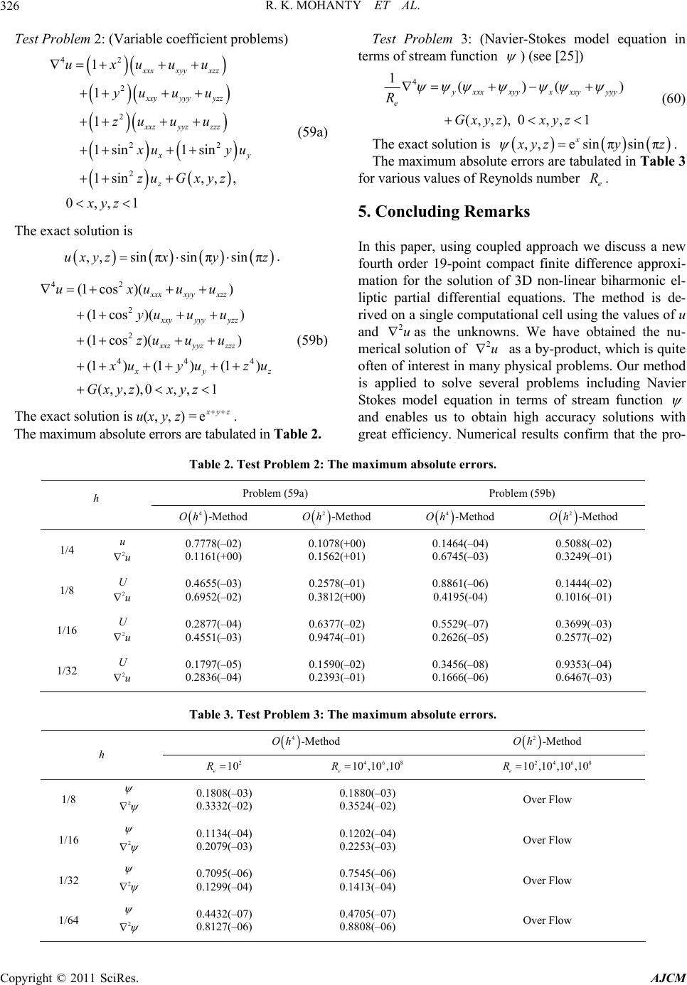

R. K. MOHANTY ET AL. 326
blems)


2
Test Problem 2: (Variable coefficient pro


 
 



42
2
2
2
1
1
1
1sin
1sin,, ,
xxx xyy xzz
xxy yyy yzz
xxz yyz zzz

2
1s
in
0,,1
x
y
z
uxuuu
yu u u
zu u u
x
uy
zu Gxyz


 
 

u
(59a)
The exact solution is
xyz


,, sinπsin πsin πuxyzx y z.
42
44
(1 cos)()
(1 co
(1 cos)()
(1) (1
(,,1
xxx xyy xzz
yyy yzz
xxz yyz zzz
2
s)( xxy
2
4
)
)
) (1
,),0 ,
x
yz
uxuuu
u u
zu u u
yu
x
uy u
Gxy z


 


zu
z xy
 
(59b)
The exact solution is u(x, y, z) =e
x
yz .
re tabulaThe m
Test Problem 3: (Navier-Stokes model equation in
terms of stream function

) (see [25])
4
1()(
(, ,),0, ,1
)
y
xxxxyyx xxyyyy
e
R
Gxyz xyz
   

(60)
The exact solution is




,, esinπsin π
x
x
yzy z  .
The maximum absolute errors are tabulated in Table 3
for various values of Reynolds number .
e
R
5. Concluding Remarks
In this paper, using coupled approach we discuss a new
fourth order 19-point compact finite difference approxi-
mation for the solution of 3D non-linear biharmonic el-
liptic partial differential equations. The method is de-
rived on a single computational cell using the values of u
and 2u

as the unknowns. We have obtained the nu-
merical solution of 2u

as a by-product, which is quite
often of interest in many physical problems. Our method
is applied to solve several problems including Navier
Stokes model equation in terms of stream function

and enables us to obtain high accuracy solutions with
great efficiency. Numerical results confirm that the pro- axm absoae 2. imulute errors ted in Tabl
em 2: The maximum absolute errors.
Problem (59a) Problem (59b)
Table 2. Test Probl
h

4-MethodOh


2-MethodOh


4-Met ho dOh

2-Met ho dOh
1/4 u 0.7778(–02)
0.1161(+00)
0.1078(+00)
+01)
0.1464(–04)
0.6745(–03)
0.5088(–02)
0.3249(–01)
2u 0.1562(
1/8 U 0.4655(–03)
0.6952(–02)
0.2578(–01)
0.3812(+00)
0.8861(–06)
0.4195(-04)
0.1444(–02)
0.1016(–01)
1/16 U 0.2877(–04)
0.4551(–03)
0.6377(–02)
0.9474(–01)
0.5529(–07)
0.2626(–05)
0.3699(–03)
0.2577(–02)
0.1797(–05)
0.2836(–04)
0.1590(–02)
0.2393(–01)
0.3456(–08)
0.1666(–06)
0.9353(–04)
0.6467(–03)
2u
2u
1/32 U
2u
Table 3. Test Problem 3: The maximum absolute errors.


4-Met ho dOh

2-Met ho dOh
h 2
10
e
R 468 10 ,10 ,10
e
R 2468 10 ,10 ,10 ,10
e
R

2

 0.1808(–03)
0.3332(–02) 0.1880(–03) 0.3524(–02) Over Flow 1/8
1/16

2

 0.2079(–0
0.1134(–04)
3)
0.1202(–04)
0.2253(–03) Over Flow
1/32

2

 0.7095(–06)
0.1299(–04)
0.7545(–06)
1413(–04) Over Flow
1/64
0.

2

 0.4432(–07)
0.8127(–0
0.4705(–07)
0.8808(–06) w 6) Over Flo

R. K. MOHANTY ET AL.327
posed fourth order method produces oscillation free so-
lution for large Reynolds number, whereas the second or-
der method is unstable.
6. References
[1] J. Smith, “The pled Equation Approach to the Nu-
merical Solution of the Bihaation by F
Differences,” SIAM Journal on Analysis, V
7, No. 1, 1970, p04-111. doi:10.1137/0707005
Cou
rmonic Equ
Numerical inite ol.
p. 1
[2] L. W. Solving the Buation as C
pled Finite Difference Equations,” SIAM Journal on Nu-
merical Analysis, Vol. 8, No. 2
doi:10.1137/0708029
Ehrlich, “iharmonic Eqou-
, 1971, pp. 278-287.
[3] L. W. EhrlichPoint and Block SOR Applied to a Cou-
pled Set of Difference Equations,” Computing, Vol. 12,
No. 3, 1974, pp. 181-194. doi:10.1007/BF02293104
, “
[4] L. Band E. L. Riess, “Bloconal Matrices
and thst Numerical Solutionrmonic Equa-
tion,” Mathematics of Computation, Vol. 26, No. 118, 1972,
pp. 311-326. doi:10.1 90/S00250312751-9
uer a
e Fa
k Five Diag
of the Biha
0 -5718-1972-
[5] R. Glowinski and O. Pironneau,
the First Biharmonic EquationsTwo-Dimen-
sional Stokes Problems,” SIAM l. 21, No. 2,
1979, pp. 167-212. doi:10.1137/1021028
“Numerical Methods for
and for the
Review, Vo
[6] Y. Kwon, R. Manohar and J. W., “Single Cell
Fourth Order Methodn,” Con-
armonic Problems,” Journal of Com-
, No. 1, 1984, pp. 65-80.
21-9991(84)90015-9
Stephenson
armonic Equatios for the Bih
gress Numerantium, Vol. 34, 1982, pp. 475-482.
[7] J. W. Stephenson, “Single Cell Discretization of Order
Two and Four for Bih
putational Physics, Vol. 55
doi:10.1016/00
y and P. K. Pandey, “Difference Methods of [8] R. K. Mohant
Order Two and Four for Systems of Mildly Non-linear
Biharmonic Problems of Second Kind in Two Space Di-
mensions,” Numerical Methods for Partial Differential
Equations, Vol. 12, No. 6, 1996, pp. 707-717.
doi:10.1002/(SICI)1098-2426(199611)12:6<707::AID-N
UM4>3.0.CO;2-W
[9] R. K. Mohanty, M. K. Jain and P. K. Pandey, “Finite Dif-
ference Methods of Order Two and Four for 2D Non
ear Biharmonic Probl
lin-
ems of First Kind,” International
Journal of Computer Mathematic s, Vol. 61, No. 1-2, 1996,
pp. 155-163. doi:10.1080/00207169608804507
R. K. Mohanty and P. K. Pandey, “Families of Acc[10] urate
Discretizations of Order Two and Four for 3D Mildly
Nonlinear Biharmonic Problems of Second Kind,” Inter-
national Journal of Computer Mathematics, Vol. 68, No.
3-4, 1998, pp. 363-380. doi:10.1080/00207169808804702
[11] D. J. Evans and R. K. Mohanty, “Block Iterative Methods
for the Numerical Solution of Two-Dimensional Nonlin-
ear Biharmonic Equations,” International Journal of C om-
puter Mathematics, Vol. 69, No. 3-4, 1998, pp. 371-390.
doi:10.1080/00207169808804729
[12] R. K. Mohanty, D. J. Evans and P. K. Pandey, “Block Ite-
rative Methods for the Numerical Solution of Three Di-
First Kind,” International Journal of Computer Mathe-
matics, Vol. 77, No. 2, 2001, pp. 319-332.
doi:10.1 010880506
mensional Mildly Nonlinear Biharmonic Problems of
080/0020716 8
[13] S. Singh and R. K. A New Cou-
pled Ap Accuracy Nethod for the
Solutioninear Biharions,” Neural
Parallel and, 2009, pp.
239-256
] D. Khattar, S. Singh and R. K. A New Cou-
pled Approachcy Numethod for the
Solution-Linear Bihuations,” Ap-
plied Mnd Compu 215, No. 8,
2009, pp. 3036-3044. doi:10.1016/j.amc.2009.09.052
, D. KhattarMohanty, “
proach High umerical M
of 2D Nonl
Scientific Computations
monic Equat
, Vol. 17
.
[14 Mohanty, “
High Accuraerical M
of 3D Non
athematics aarmonic Eq tations, Vol.
w High Accuracy Finite Difference
Discretization for the Solution of 2D Non-Linear Bihar-
monic Equations Using Coupled Approach,” Numerical
Methods for Partial Differential Equations, Vol. 26, No.
4, 2010, pp. 931-944. doi:10.1002/num.204605
[15] R. K. Mohanty, “A Ne
Mohanty, M. K. Ja. Mishra, “A Com-
t Discretization of O(h) for Two-Dimensional Non-
ear Triharmonic Equations,” Physica Scripta, Vol. 84,
. 2, 2011, pp. 025002.
/0031-8949/84/02/025002
[16] R. K.
pac
in and B. N
4
lin
No
doi:10.1088
K. Mohanty and S. Deyell Fourth Order Dif-
ence Approximations for (  u/  x), (  u/  y) and (  u/  z)
the Three Dimensional Quasi-Linear Elliptic Equation,”
merical Methods for fferential Equations,
, No. 5, 2000, pp. 417-425.
[17] R. , “Single C
fer
of
Nu
Vol. 16
Partial Di
doi:10.1002/1098-2426(200009)16:5<417::AID-NUM1>
3.0.CO;2-S
[18] R. K. Mohanty, S. Karaa and U. Arora, “Fourth Order Nine
artial Differential Equations,” Nume-
Point Unequal Mesh Discretization for the Solution of 2D
Non-Linear Elliptic Partial Differential Equations,” Neu-
ral Parallel and Scientific Computations, Vol. 14, 2006,
pp. 453-470.
[19] R. K. Mohanty and S. Singh, “A New Highly Accurate Dis-
cretization for Three Dimensional Singularly Perturbed
Non-linear Elliptic P
rical Methods for Partial Differential Equations, Vol. 22,
No. 6, 2006, pp. 1379-1395. doi:10.1002/num.20160
[20] L. A. Hageman and D. M. Young, “Applied Iterative Me-
thods,” Dover Publications, New York, 2004.
[21] M. K. Jain, “Numerical Solution of Differential Equa-
tions,” 2nd Edition, John Wiley, New Delhi, 1984.
[22] C. T. Kelly, “Iterative Methods for Linear and Non-Linear
Equations,” SIAM Publications, Philadelphia, 1995.
[23] Y. Saad, “Iterative Methods for Sparse Linear Systems,”
SIAM Publications, Philadelphia, 2003.
doi:10.1137/1.9780898718003
[24] G. Meurant, “Computer Solution of Large Linear Systems,”
North-Holland, Amsterdam, 1999.
[25] W. F. Spotz and G. F. Carey, “High Order Compact Scheme
for the Steady Stream-Function Vorticity Equations,” In-
ternational Journal for Numerical Methods in Enginee-
ring, Vol. 38, No. 20, 1995, pp. 3497-3512.
doi:10.1002/nme.1620382008