American Journal of Computational Mathematics, 2011, 1, 303-317
doi:10.4236/ajcm.2011.14037 Published Online December 2011 (http://www.SciRP.org/journal/ajcm)
A Gas Dynamics Method Based on the Spectral Deferred
Corrections (SDC) Time Integration Technique and the
Piecewise Parabolic Method (PPM)
Samet Y. Kadioglu
Fuels Modeling and Simulation Department, Idaho National Laboratory, Idaho Falls, USA
Received September 8, 2011; revised November 1, 2011; accepted November 8, 2011
Abstract
We present a computational gas dynamics method based on the Spectral Deferred Corrections (SDC) time
integration technique and the Piecewise Parabolic Method (PPM) finite volume method. The PPM frame-
work is used to define edge-averaged quantities, which are then used to evaluate numerical flux functions.
The SDC technique is used to integrate solution in time. This kind of approach was first taken by Anita et al
in [1]. However, [1] is problematic when it is implemented to certain shock problems. Here we propose sig-
nificant improvements to [1]. The method is fourth order (both in space and time) for smooth flows, and pro-
vides highly resolved discontinuous solutions. We tested the method by solving variety of problems. Results
indicate that the fourth order of accuracy in both space and time has been achieved when the flow is smooth.
Results also demonstrate the shock capturing ability of the method.
Keywords: Gas Dynamics, Conservation Laws, Spectral Deferred Corrections (SDC) Methods, Piecewise
Parabolic Method (PPM), Godunov Methods, High Resolution Schemes
1. Introduction
In this paper, we present a conservative scheme based on
the SDC and PPM methods. The integration of the SDC
method to the PPM method was first carried out by Anita
et al in [1]. However, [1] is problematic in the sense that
it is oscillatory when it is applied to certain shock prob-
lems unless complicated extra repair steps are introduced.
The oscillations are developed around the shocks at ear-
lier times, then spread into entire computational region.
These oscillations are neutral oscillations (extraneous
wiggles) that pollute the solution and never disappear.
The main reason for having such wiggles is that the PPM
fluxes (without the time averaging in SDC framework)
are evaluated in a way to obtain sharper discontinuous
profiles, therefore lack of necessary numerical diffusion
mechanism. Here, we introduce a strategy that eliminates
the oscillatory behavior of [1].
The SDC-PPM method falls in to the class of higher
-order high-resolution-schemes. Here, we shall provide a
short historical perspective to higher-order high-resolu-
tion-schemes. High resolution schemes are designed to
solve gas dynamics equations (Gas dynamics equations
are also referred to as the inviscid Euler equations or the
conservation laws. Hereafter, we will use all of three
terminologies interchangeably). In the last several dec-
ades, many numerical schemes were introduced for this
purpose. Godunov [2] initiated a novel approach that is
now accepted as one of the main building blocks for
construction of a high resolution scheme. Godunov sup-
posed that the initial data could be replaced by a piece-
wise constant set of states (i.e, cell averages of the initial
solution) with discontinuities located at computational
cell edges (cell faces in 3-D). He then found exact solu-
tions to this simplified problem by locally performing the
well-known Riemann solution theory. Finally, he re-
placed exact solutions by a set of piecewise constant ap-
proximations (i.e, exact solutions are averaged down to
the local cells). Godunov’s method revolutionized the
field of computational gas dynamics, by overcoming
many of the difficulties that have been persistent for
many years. However, Godunov’s method was only first
order accurate. The first major improvement to Godunov’s
work was made by van Leer [3] who approximated the
initial data and solutions at each subsequent time level by
piecewise linear segments allowing discontinuities be-

S. Y. KADIOGLU 304
tween the segments. Van Leer’s work, also known as the
MUSCL (Monotonic Upwind Scheme for Conservation
Laws) scheme, raised the order of accuracy of the Go-
dunov’s method to two. Later, van Leer’s MUSCL
scheme was reconsidered or revised by others [4-6]. For
instance, Colella’s MUSCL scheme [5] defines the
slopes for the linear reconstruction based on the average
values as oppose to van Leer [3] treats them as separate
variables. When the flow is smooth, Colella’s slope defi-
nition corresponds to a fourth order finite difference ap-
proximation to the derivative of a given state variable.
Colella’s work [5] was another step forward to increase
the accuracy of the Gudonov’s method. So far the
Godunov type methods used constant or linear piecewise
reconstructions. In [7], Colella and Woodward intro-
duced a new method which is based on a piecewise
parabolic reconstruction of solutions. Their method, fa-
mously known as the Piecewise Parabolic Method (PPM),
achieves more accurate (fourth order in space) solution
representations for smooth flows as well as it captures
steeper shock discontinuities.
The MUSCL schemes [4-6] or the PPM method [7]
are the few examples of higher order high-resolution-
schemes. There exists number of other high-resolution
schemes such as ENO[8], WENO[9], TVD[10], FCT[11],
PHM[12], and LLR[13,14] methods. In several instances,
comprehensive studies have been carried out to compare
the performance of these schemes [15-19]. We remark
that these above cited studies mostly favor the PPM
method. A particularly attractive feature of PPM method
is that it can produce fourth order accurate calculations
as long as the solutions stay smooth. We exploited this
aspect when we studied zero Mach number flow prob-
lems (our collaborated work with M. Minion in [20]).
The drawbacks of the PPM method reveal mostly when it
is applied to shock problems. For instance, the PPM
method [7] needs several external repairs in order to
produce discontinuous solutions without spurious oscil-
lations. The oscillatory behavior is associated with the
method not having enough numerical diffusion (dissipa-
tion). In order to add appropriate numerical diffusion, the
fluxing steps are modified in a way that the so-called
smoothening and flattening algorithms have to be per-
formed. We note that the implementation of these addi-
tional steps can be complicated. In our work, we avoid
these external fixes by using a rather simple approach
which will be explained next.
The SDC method is based on a number of deferred
corrections of a low order provisional solution, which is
predicted by forward or backward (depending on the
stiffness of the problem) Euler method in order to
achieve higher order of accuracy in time. In our case, we
perform three deferred corrections to obtain fourth order
accurate solutions. The SDC-PPM method of [1] uses the
PPM fluxing procedure to evaluate the numerical flux
functions and employs the SDC method to integrate so-
lutions in time. We observed that the SDC-PPM method
develops neutrally stable oscillations at the prediction
step and maintains these oscillations during the deferred
correction iterations. The main reason for this behavior
(as mentioned above) is that the higher order flux evalua-
tion at the prediction step lacks of necessary numerical
diffusion so as the correction steps leading to unwanted
oscillations around discontinuities. We fix this behavior
with the following strategy. We know from our observa-
tion that one has to use more diffusive fluxes at the pre-
diction step to avoid potential oscillations. Thus instead
of full PPM fluxing, we employ an up-winding proce-
dure that is naturally more diffusive. On the other hand,
we let the correction iterations include the higher order
PPM fluxing. With this strategy, we found out that solu-
tions from the prediction step have enough numerical
diffusion so that potential oscillations that might come
from the correction steps are killed off. One question
about this strategy is that does the up-winding procedure
excessively smear the discontinuities? Our finding indi-
cates that although the shocks are smeared at the predic-
tion step, the correction iterations sharpen them back. In
fact, we have obtained the same sharpness (and same
shock amplitudes in that matter) as the full PPM would
predict. We remark that the full PPM method [7] as well
as the SDC-PPM method [1] has to make use of the
smoothening, flattening, and artificial diffusion steps in
order to keep solutions oscillation free. We avoid all of
these extra steps in our approach.
The organization of this paper is as follows. In Section
2, the governing equations are presented. In Section 3,
some notational conventions and the numerical algorithm
are described. In Section 4, the computational results are
presented. In Section 5, our concluding remarks are
given.
2. Governing Equations
The in viscid Euler partial differential equations are
widely used to model gas dynamics problems. These
equations describe the physical evolution of conserved
quantities such as mass, momentum, and total energy in
space and time. Therefore, they are often referred to as
the conservation laws. The conservation laws fall into
class of the hyperbolic partial equations that admit dis-
continuous solutions such as shock waves. Therefore
these equations are the best model for a gas problem in
which shock waves frequently occur.
We consider the following two dimensional conserva-
tion equations,

S. Y. KADIOGLU305
 
0,
FU GU
U
tx y


  (1)
where U is the vector of conserved quantities, and F(U)
and G(U) are the flux functions in x- and y-directions. For
instance,
,
u
Uv
E











2
,
u
up
FU uv
Epu












and


2,
v
uv
GU vp
Epv












where and E denote density, velocity, pres-
sure, and the total energy. E satisfies

,,,uv p 

22
1.
12
p
Eu 

 


v (2)
This equation is called the equation of state for an ideal
polytropic gas. An ideal gas obeying (2) is also referred to
as the gamma-law gas with

denoting the specific heat
ratio. Under ordinary circumstances air is composed
primarily of 2 and 2, so N O1.4

. We will use
1.4

 in all of our computations.
3. Numerical Algorithm
3.1. Notations and Formulation
In this section, we briefly review several notational con-
ventions that we have introduced in [20]. For ease of
presentation, we assume that the physical domain is
two-dimensional and divided into a uniform array of cells
of width and height h. Let the cell with center at

,
ij

x
ybe denoted by the pair (i, j), and let the half integer
subscripts i+ 1/2 and j + 1/2 denote a shift by distance h/2
in the x- and y-direction respectively. The extension to
rectangular cells and three dimensions is straightforward.
The PPM method or many other high resolution
schemes rely on the so called finite-volume approach. The
finite-volume approach is based on the evolution of cell
averages. A cell average for some quantity

,,
x
yt  is
defined by


12 12
12 12
2
1
,, ,,dd.
ij
ij
xy
ij
xy
x
ytxyt yx
h



 (3)
Similarly, cell edge averages of a quantity


,,
x
yt 
are defined as

12
12
12 12
1
,, ,,d,
j
j
y
ij i
y
x
ytxyt y
h





 (4)
and

12
12
12 12
1
,, ,,d.
i
i
x
ij j
x
x
yt xytx
h





 (5)
Figure 1 gives a graphical illustration of the above
definitions. To specify the finite volume formulation of
the conservation law


.
t
UFU0

 (6)
where


,,Uxyt is the vector of conserved quantities
and F(U) =






,
F
UGU is the flux function (notice
that Equation (6) is equivalent to Equation (1)), we inte-
grate Equation (6) over the computational cells and use
the divergence theorem to attain
  
2
,
1
,,,, 0
t
ij
Uxyt FUxyt
h


 (7)
where the flux integral above is defined as

   
   
12
12
12
12
12 12
,
12 12
,,,, d
,,,,d
j
j
i
i
y
ii
ij y
x
jj
x
F
UFUxytFUxyt
GU xytGU xytx










y
(8)
Using the definitions of the edge average in Equation
(4)-(5)
,12ij



12,ij



,ij

Figure 1. Cell and cell-edge averaged representation of a
quantity

.

S. Y. KADIOGLU 306
 



 

   

,
12 12
12 12
,,
,, ,,
,, .,
ij
ij ij
ij ij
FU xyt
hFUxy tFUxy t
hGU x ytGU xyt








.
(9)
Therefore,

   
   
12 12
12 12
,,
,, ,,
,, ,,
0.
tij
ij ij
ij ij
Uxyt
FUxytFUxy t
h
GU xytGU x yt
h








(10)
Furthermore, if we let

,,
iji j
UUxyt,
 
12, 12
,,
iji j
F
FU xyt


 and
  

,12 12
,,
iji j
GGUxyt


 
, then we arrive at
12,12,, 12, 120. ij ijijij
ijt
FFGF
Uhh
 



 
 (11)
3.2. The Fourth Order Spectral Deferred
Corrections (SDC) Time Integration
Algorithm
The construction of stable and accurate numerical meth-
ods for solving initial value problems is a well studied
subject [21-23]. Runga-Kutta methods or linear multi-step
methods are highorder discretization schemes by con-
struction. On the other hand, Richardson extrapolation or
deferred correction methods are based on increasing the
accuracy of a low order method through iterations. The
second group is also known as the predictor-corrector
techniques. High order direct discretization schemes can
be expensive due to the stability constraint. In this case,
most practitioners recommend the predictor-corrector
techniques.
In this paper, we consider the spectral deferred correc-
tions method. The spectral deferred corrections (SDC)
method, introduced in [24], is a known stable numerical
technique with, in principle, arbitrarily high order of ac-
curacy. The SDC method proceeds by first using a simple
low order numerical method to compute a provisional
(predicted) solution at a set of sub-steps within a given
time step. Then, an equation for the correction to this
provisional solution is constructed and also approximated
on the sub-steps with the same numerical scheme. Each
iteration at the correction step increases the accuracy of
the provisional solution by one.
We briefly describe the SDC procedure here, for details
see [24-26].
Consider the initial value problem,






,tF tt 



,tab, (12)


a
a



(13)
The SDC method is based on the observations con-
cerning the integral form of the solution to Equations
(12)-(13)
  
,d.
t
a
a
tF

 



(14)




,,d
t
a
a
Et Ft    

 (15)
Since






tt  

t
t, Equation (14) is simply
  

,d
a
a
tt F



  


, (16)
which then can be combined with Equation (15) to give
 




(),,d
,.
t
a
tF F
Et

  









(17)
This equation is referred to as the correction equation.
Now given Equations (12) and (13) and time interval


1
,
nn
tt

in which the solution is desired, the SDC
method proceeds by first di

viding

1
,
nn
tt
 into p subin-
tervals by choosi points 0m ng forp
, with
1pn
m
t..
012n
tttt tt


 (18)
Here, the interval


1
,
nn
tt

will be referred to as a time
step while a subinterval




1
,,
mmmm m
tt t
tt will be
referred to as sub step. Then an approximate solution


0
m
t  is computed for using a standard
forward Euler method. Next, a sequence of corrections
0mp


k
m
t  is computed by approximating Equation (17) to
provide an increasingly accurate approximation to the
solution 1kkk





. To achieve this, the function




,t
k
Et 
in Equation (17) must be calculated with
spectral accuracy, i.e, by a Gaussian quadrature. Our
choice of quadrature nodes is the Gauss-Lobatto nodes.
This is because the Gauss-Lobatto nodes already include
the end points, therefore, one does not have to do ex-
trapolations of the final solution to those points. See [25]
for different choices of quadrature nodes.
A discretization for Equation (17) based on the forward
Euler method is given by

 
 
1
1
,,
,
kkkk k
mmm mmmmm
kk
mm
tFt Ft
EE
 





 


 (19)
where


kk
mm
t  ,


kk
m
t  m and




,
kk
mm
EEt  .
m
Each iteration for Equation (19)

S. Y. KADIOGLU 307
raises the formal temporal order of accuracy of the
scheme by one, therefore for a fourth order method, three
iterations (e.g, k = 3) of the correction equation are
needed. Also, for a fourth order method, four Gauss-
Lobatto points are necessary, i.e, p = 3 in Equation (18).
Now reconsider Equation (11) in the following form

,
ijt ij
UfUt (20)
where

12,12,, 12, 12
,.
ij ijijij
ij
FFGF
fUthh
 

 
  
Here we skipped the bar convention, but ij Uill al-
ways represent cell averages. Let ,
k
ij m
Uresent the nu-
merical solution of Equation (20) at th
ms step and th k
ate. Then the SDC algorithm can be summarized as:
B
w
rep
ub
iter asic structure of the SDC algorithm:
e Lints, in
While tt final
Define thobatto po01 3 ,, ,tt t


1
,
nn
tt

,
Define

1
,0ij n
UUt
ij
on step: Predicti
Compute the provisional solutions using the forward
Eu
for orrection sp:
onal solutions by solving the cor-
re


1
,1 ,
,, ,
,,1,
,,
,d
m
m
kk
ij mij m
kkk
mij mij mmij mm
t
kkk
ij mij mij m
t
tfUtfUt
fUUU














1
,1,1 ,1
,
kkk
ij mij mij m
UU 





for 0,, 2m
end
Copy


4
1,ni
ij
Ut U
3j
End
3.3. The Fourth Order PPM Oriented Flux
Calculations
In this section, we define the cell edge averaged quantities
that will be used to calculate the numerical flux functions,
i.e, 12,ij and F

,12ij
G
 in (11) or in (20). The procedure
is based on Colella and Woodward [7]. In [7], cell edge
averages are calculated by interpolating quartic polyno-
mials which are constructed through cell averages. For-
mulae, in [7], are given for one dimensional non-equally
spaced mesh. The formulae below are the two dimen-
sional versions of [7] in a uniformly spaced mesh. Below,
we systematically describe the steps to calculation of
12,ij and
ler method, i.e,
1
U

1 1
,1 ,,
,,
ijmijmmijm m
UtfUt

0,, 2m
C teF

,12ij
G
. First, evaluating the interpolation
functions ( the construction of interpolation functions and
more detail can be found in [7]) at the

12, th ij
Correct the provisi
ction equation for three iterations,
for k = 1, 3

and

,12
th
ij

edges of cell gives the following
edge formulae:

,th ij
set ,00
k
ij
 
 
12,1, ,,1,
11
ˆ
26
xx
iji jijijij
UUU UU 


x

(21)
 
,12,1,,,1
11
ˆ
26
yy
ijij ijijij
UUU UU 


y

(22)
where

1, 1,1,,,1,
,
1
sgn if0
2
0otherwise
x
ijij ijij ij ij ij x
ij
UU UUUU
U


 

,








(23)
1, 1,1,,, 1,
1
min, 2, 2,
2
x
iji jiji jijijij
UU UUUU 
 

 


(24)

,1 ,1,1 ,,,1
,
1
sgn if0
2
0otherwise
y
ijij ijijijijij
y
ij
UU UUUU
U


 

,








(25)
,1 ,1,1 ,,,1
1
min, 2, 2.
2
y
ijij ijijijijij
UU UUUU 
 

 


(26)

S. Y. KADIOGLU 308
Equations (21) and (22) are the slope limited edge
quantities. Notice that if


,1,
12
x
iji jij
UUU 


1,
,
then Equation (21) simplifies into
1, 7
ˆij
xUU
U

)
,1,2, . ijiji j
UU

  (27
Similarly if
12 ,12 ij 

,,1,
1
2
y
ijij ij
UUU 


1
then
(22) becomes
Equation
,1,,1, 2
,12
ˆ.
j
y
ij
U


 (28)
7
12
ijij iji
UUUU

 
Equations (27) and (28) are fourth order extrapolations
to the edge quantities. Consequently, this mak
scheme fourth order accurate in space in regions where
th
es the PPM
e solution is smooth. To prevent possible overshoots or
undershoots, the slope limited edge quantities are further
monotonized with the monotonicity algorithm.
Monotonicity algorithm:
Initialize
12,
,1,
LR
ij
ij i j
ˆ,
x
UU U ,12
,,1
ˆ
LR
y
ij
UU U
ij ij 
 (29)
Modify

,,
,,
,,
,,
,,
if 0,
LR
RL
ij ij
ij ij
ij ij
ij ij
UUUU
UUUU

 
(30)

,,
,,
,,
,,
,,
if 0,
LR
RL
ij ij
ij ij
ijij
ij ij
UUUU
UUUU

 
(31)


,
,,
,
,, ,,
2
,,
32,
1
if 2
,
6
LR
RL RL
RL
ij
ij ij
ij
ij ijij ij
ij ij
UUU
UUU UU
UU










(32)


,
,,
,
,, ,,
2
,,
32,
1
if 2
,
6
LR
RL RL
RL
ij
ij ij
ij
ij ijij ij
ij ij
UUU
UUU UU
UU







(33)


,
,,
2
,,
,
,, ,,
32,
if 6
1,
2
RL
RL
RL RL
ij
ij ij
ij ij
ij
ij ijij ij
UUU
UU
UUUUU




 




,
,,
2
,,
,
,, ,,
32,
if 6
1.
2
RL
RL
RL RL
ij
ij ij
ij ij
ij
ij ijij ij
UUU
UU
UUU UU




 


(35)
We note that the aim is to construct the Riemann vari-
ables, with which the numerical flux functions are evalu-
ated. To define the point-wise Riemann variables, first
we set
12,12,, 12
,1,
,12
,,1
,,
,.
RL
RL
LR
ij ijij
ijij
R
ij
ij ij
UUUUU
UU U





L

(36)
Then the slope limited and monotonized corner points
at each direction can be calculated through following
Equ ations (21)-(35). At this point we have the right/left
corner values, i.e,
,,,,
12,1212,1212,1212,12
,,,and.
LyRy LxRx
ij ij ijij
UUU U
  
Now we can define the Riemann variables along cyell
edges by taking the two corner values and a cell edge
averaged quantity. First we construct a quad
nomial along each cell edges. For instance, along the
ratic poly-

12,jedge, for given
th
i,,
12,1212, 12
,
Ly Ly
ij ij
UU
  and
12,
L
ij
U, we determine the coefficients of the quadratic
polynomial (i.e.,


2
Uyayby c

) with,
,
12,
Ly
ij
U

22
1212 12 j j
aybyc
 
 (37)


12
12
12,d
j
ij
y
UUyy
h
 (38)
1j
y
L

,22
12,121212
Ly
ijj j
Uaybyc


 (39)
structing the quadratefine
o left point-wise Riemann variables at the two
Gauss points, i.e.,
After conic polynomial, we d
the tw
for , in
12
,yy 12 12 , interval,
jj
yy



c
,22
111
,
Ly
Uayby


c
(40)
,22
222
.
Ly
Uayby

 (41)
The right point-wise Riemann variables, ,
1
R
y
U, ,
2
R
y
U
can be defined similarly.
Using these Riemann variables, we calc
mann solutions at the two Gauss points, i.e.
ulate the Rie-
,


,,
111
,,
yRimLyRy
UU UU

,,
222
,,
yRimLyRy
UU UU (42)
where


,
R
imL R
UUU sents solution. repre the Riemann
An exann solution to
tions will be given below.
Finally, using these point-wise Rie
calculate the average F flux along the
(34) ample of a Riem the Burgers equa-
mann solutions, we

12, th ij cell

S. Y. KADIOGLU309
edge as,
 
12
12,.
2
ij
FU FU
F


 (43)
yy
Similarly we calculate Gfluxes along the

,12
th
ij cell edges usg Equations (37)-(42) with
d by x, i.e.,
in y
replace
 
12
. (44)
g the SDC
t the numerical variables representing cell av-
erages and cell edge fluxes are always computed at the
same time level (i.e. there is no time-ce
as in most second-order Godunov type schemes).
A Riemann
,1 22 ij
Remark: One observation about usinstrat-
egy is tha
xx
GUGU
G 

ntering of fluxes
Solution to the Burgers Equation
Consider,
22
11
0. (45)
22
t
xy
uu u




Characteristics speed in both x and y directions is u,
i.e., d
d
xu
t and d d
yu
t. Thus we have to consider the
following four cases in both coordinate directions.
x-direction:
Case 1: If
L
u and , then the wave (either shock
herefore
n solution becomes
.
0
R
u
or rare-faction wave) moves from left to right. T
the Rieman

,
R
imL RL
uuuu (46)
Case 2: If
L
u and 0
R
u, then the wave (either
ock or rare-factioe) moves from right to left. shn wav
efore thann soThere Riemlution becomes

,.
R
imL RR
uuuu (47)
Case 3: If0
L
R
uu, t
0.
 hen we have a rare-faction
wave. Therefore the Riemann solution becomes

,
RimL R
uuu

(48)
Case 4: If 0
L
R
uu
is
then we
Th b
have a shock wave.
e shock speed calculated y
 
.
2
LR
L
R
LR
Fu Fuuu
suu


 (49)
Then the Riemann solution is giv
The Riemann solution in y-dir
milarly.
e employ a
words, we define the
left and right values in (36) by using the left and right
state of the solution vector, e.g.,
en by

if 0
,if0,
L
Rim
R
us
uuuus


 (50)

L R
ection is calculated si-
Remark: Wn up-winding flux procedure at
the SDC’s prediction step. In other
12,, , ij
U
L
ij
U

12,1,
R
ij ij
x evaluation for Equations (43) and (44).
UU

. This provides more diffusive numerical
flu
4. Numerical Results
4.1. Solving the Linear Advection Equation
We consider,
0,
txy
uu u

 01,01xy  (51)
As a first test, we use a smooth initial solution;




,,0 sin2π2cos 2π.xyx y (52)
In this test, the solution stays smooth i
u
n time. We
monstrate the fourth order of
periodic boundary
otice
sim-
) and (28). Also one doesn’t have to apply
ity algorithmr this specific test case.
Figure 2 shows the orm of the absolu
die indi-
cating the stability of the de-
creases by the factor ofen for a finer me
in
solve this test problem to de
accuracy of our method. We apply
conditions in both x and y-coordinate directions. N
that the edge average formulae for the state variable
plifies into (27
the monotonic fo
nte error for
2
L
sixte
fferent meshes. The error grows linearly in tim
numerical scheme, and
sh indicat-
g the fourth order convergence. Tables 1-3 show the
convergence rates with different norms. The convergence
rate

is estimated using the two finest grids according
to the following formula


error
1ln .
ln 2error2
x
x







(53)
Figure 2. Demonstrating the fourth order of accuracy of the
method with the L2-norm when solving Problem (4.1).

S. Y. KADIOGLU 310
Table 1. Error table in terms of max norm for the linear ad-
vection Problem (4.1). The final time is set to. Here
the solution uses the smooth initial Function (52).
Mesh
refinement
1.0t
max
exact num
uu
h = 1/10 9.43
Between mesh Convergence
rates
2
10 
h = 1/20 6.18 1/10 - 1/20 3.93
3
10 
h = 1/40 3.94 1/20 - 1/40 3.97
h = 1/80 2.48 1/40 - 1/80 3.98
4
10 
5
10 
Table 2. Error table in terms of norm for the linear ad-
vection problem (4.1). The final is set to. Here
the solution uses the smooth initial Function (52).
Mesh
1
L
time 1.0t
refinement 1
exact num
L
uu
h = 1/10 4.30 2
10 
Between
mesh
Convergence
rates
h = 1/20 2.82 3
10  1/10 - 1/20 3 3.9
h = 1/40 1.78 4 10  1/20 - 1/40 3.98
1.11 1/40 - 1/80 h = 1/80 5 10  4.00
Tabr ta terms of the -
veblem ). The final time is set toHere
the usessmooh initn (52).
refinement
le 2. Erro
ction Proble in (4.12
L norm forlinear ad
1.0 . t
solution the tial Functio
Mesh
2
exact num
L
uu
h = 1/10 5.04 2
10  mesh rates
Between Convergence
h = 1/20 3.293 10  1/10 - 1/20 3.93
h = 1/40 2.08 1/20 - 1/40 3.98
1.30 1/4
4
10 
h = 1/80 5
10  0 - 1/80 4.00
Ta -3 also indicate the fourth order of accuracy
of od. When performingergenaly-
sis set to equal to
bles 1
our meth the convce an
, t is


x
y

 and thes
refinehalf for consecutive r
Iond te slve E1) wi ini-
al discontinuity, i.e.,
in th doubly period domain. Figure 3 illustrates
the solution after one perod iig
duc g
mesh i
d uns.
n the secest, woquation (5th an
ti

1.0if 0.30.7,0.30.7
,,0 0.0 otherwise,
xy
uxy 


 (54)
e sameic
in time. Fure 3 is pro-
ed usin 180xy and early,
wee aner/under sindi-
cating thPPMuxing proceorks qu
4.2. Solving the Burgers E
4.
0.5tx 
e solu
. Cl
don’t sey ovhoots in thtion
at the fldure wite well.
quation
2.1. 1-D Burgers Test Problem
We consider the one dimensional Burgers equation;
Figure 3. Propagation of the initial square pulse after one
uta- period (t = 1.0). 80 grid points are used for this comp
tion.
2
10,
2
t
x
uu




 (55)
with




0
,0 .uxu x
sidered in [27,15] and follows
The following test case is con-
as setting the initial solu-
tion to a smooth parabolic profile. For instance,
 

0
max 0,1if0.0.
if 0.0
o
yy y
uy uy y






(56)
where y = 5x − 2.5 and x belongs to [0, 1]. Periodic
boundary conditions are applied at both x = 0 and x = 1.
At t = 0.2, shock waves start forming in the solution nea
x = x =
r
0.3 and 0.7. After this time, the shock waves
propagate in the solution with

1.
2LR
s
uu
To be consistent with [15], we use the same number of
grid points (e.g., 40) to produce o
sults. The time stepping criteria
cept omitting the c, since the only characteristic speed is
lution u itself. W
ning the
code with 200 grid points. Comparing our results to the
results reported in [15], we observed that our r
better or comparable to the most of the high res
schemes (e.g., ENO, WENO, FCT, PPM, TVD-MUSCL
urgers equation;
ur computational re-
uses Equation (59) ex-
the soe set cfl = 1.0 in (59). Figure 4
represents the computed solutions at t = 0.5 and t = 2.4.
The reference solutions are calculated by run
esults are
olution
etc). Notice that there is no over/under shoots around the
shock profiles.
4.2.2. 2-D Burgers Test Problem
We consider the two dimensional B
22
0, 01, 01
22
txy
uuuxy

11



 (57)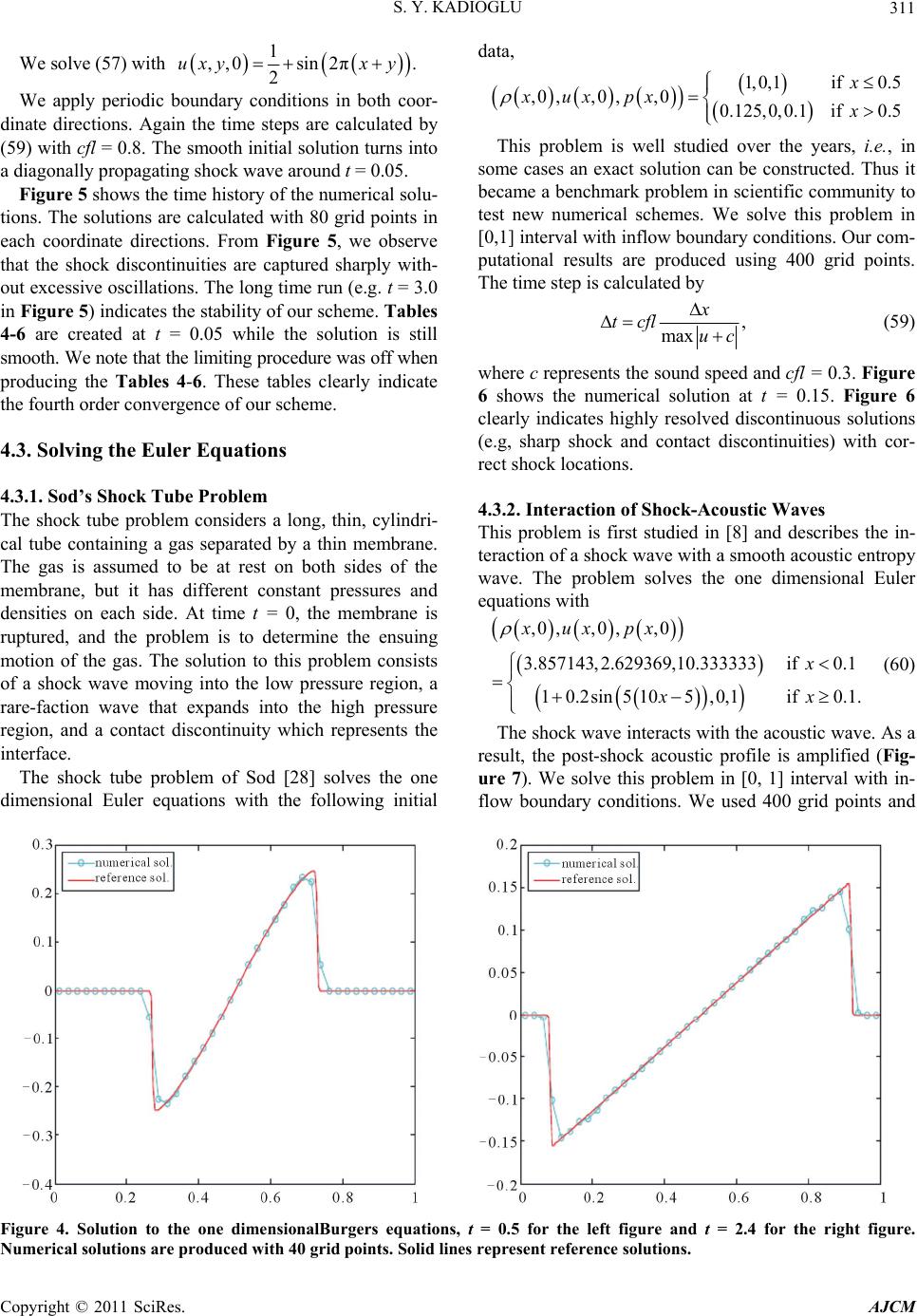

S. Y. KADIOGLU 311
We solve (57) with
 

1
,,0 sin2π.
2
uxyxy
We apply periodic boundary conditions in both coor-
dinate directions. Again the time steps are calculated by
(59) with cfl = 0.8. The smooth initial solution turns into
a diagonally propagating shock wave around t = 0.05.
Figure 5 shows the time history of the numerical solu-
tions. The solutions are calculated with 80 grid points in
each coordinate directions. From Figure 5, we observe
that the shock discontinuities are captured sharply with-
out excessive oscillations. The long time run (e.g. t = 3.0
in Figure 5) ind
data,
 


1, 0,1if0.5
,0 ,,0 ,,00.125,0,0.1 if0.5
x
xux pxx






This problem is well studied over the years, i.e., in
some cases an exact solution can be constructed. Thus it
became a benchmark problem in scientific community to
test new numerical schemes. We solve this problem in
[0,1] interval with inflow boundary conditions. Our com-
putational results are produced using 400 grid points.
The time step is calculated by
,
max
x
tcfl uc

  (59)
icates the stability of our scheme. Tables
the solution is still
hen
cate
the fourth order convergence of our scheme.
4.3. Solving the Euler Equations
4.3.
4-6 are created at t = 0.05 while
smooth. We note that the limiting procedure was off w
producing the Tables 4-6. These tables clearly indiwhere c represents the sound speed and cfl = 0.3. Figure
6 shows the numerical solution at t = 0.15. Figure 6
clearly indicates highly resolved discontinuous solutions
(e.g, sharp shock and contact discontinuities) with cor-
rect shock locations.
1. Sod’s Shock Tube Problem
The shock tube problem considers a long, thin, cylindri-
cal tube containing a gas separated by a thin membrane.
The gas is assumed to be at rest on both sides of the
membrane, but it has different constant pressures an
4.3.2. Interaction of Shock-Acoustic Waves
This problem is first studied in [8] and describes the in-
teraction of a shock wave with a smooth acoustic entropy
wave. The problem solves the one dimensional Euler
equations with
d
densities on each side. At time t = 0, the membrane is
ruptured, and the problem is to determine the ensuing
motion of the gas. The solution to this problem consists
of a shock wave moving into the low pressure region, a
rare-faction wave that expands into the high pressure
region, and a contact discontinuity which represents the
interface.
The shock tube problem of Sod [28] solves the one
dimensional Euler equations with the following initial









 

,0 ,,0 ,,0
3.857143,2.629369,10.333333 if0.1
10.2sin5105,0,1 if0.1.
xux px
x
xx






(60)
The shock wave interacts with the acoustic wave. As a
result, the post-shock acoustic profile is amplified (Fig-
ure 7). We solve this problem in [0, 1] interval with in-
flow boundary conditions. We used 400 grid points and
Figure 4. Solution to the one dimensionalBurgers equationst = 0.5 for the left figure and t = 2.4 for the right figure.
Numerical solutions are produced with 40 grid points. Solid lines represent reference solutions.
,

S. Y. KADIOGLU 312
Figure 5. The time evolution of the solution to the 2-D Burgers equation. t = 0.0 for the top, t = 1.0 for the middle, anf t = 3.0
for the bottom figures. Figures on the right are the diagonal cuts of the left ones. 80 × 80 mesh is used to produce these re-
sults.

S. Y. KADIOGLU 313
Table 4. Error table in terms of norm for Problem
(4.2.2). The final time is set to 1
L
0.05t

. Table 6. Error table in terms of max norm for Problem (4.2.2). The final time is set to .
Mesh
refinement
0.05t
Mesh
refinement 1
2hh
L
uu 2max
hh
uu
2h = 1/20 1.60
Between
mesh
Convergence
rates Between mesh Convergence rates
2h = 1/20 7.20
3
10  3 10


2h = 1/40 1.25 1/20 - 1/40 3.67 2h = 1/40 1.60 1/20 - 1/40 2.16
4
10  3 10


2h = 1/80 9.01 1/40 - 1/80 3.79
2h = 1/160 6.31 1/80 - 1/160 3.83
2h = 1/80 1.75
6
10 
7
10 
4
10

 1/40 - 1/80 3.19
2h = 1/1601.47 5
10

 1/80 - 1/160 3.57
Table 5. Error table in terms of norm for Problem
(4.2.2). The final time is set to 2
L
0.05t

.
Mesh
refinement 2
2hh
L
uu
2h = 1/20 2.50
Between
mesh
Convergence
rates
3
10 
2h = 1/40 3.58 1/20 - 1/40 2.80
4
10 
2h = 1/80 2.85 1/40 - 1/80 3.65
2h = 1/160 2.11 1/80 - 1/160 3.75
5
10 
6
10 
cfl = 0.3 in (59) to generate our results. The reference
solution is produced with 1600 grid points. Figure 7
shows our computational result. We obtained highly re-
solved solution comparable to [8] and [12,14]. This is an
important problem to study, since the solution has some
structure in the smooth region. As noted in [8], higher
order methods perform better in such regions. Our results
confirm this. In other words, our results are comparable
to higher order ENO [8], higher order PHM (Piecewise
Hyperbolic Methods) [12], or higher order LLR (Local
Figure 6. Sod’s shock problem.

S. Y. KADIOGLU 314
Figure 7. Shock-acoustic wave pro b le m . t = 0.18.
Logarithmic Reconstructions Method) yet better than the
second order MUSCL-type schemes.
4.3.3. Interaction of Blast Waves
This problem is introduced by Woodward and Colella
[17] and is often referred to as the Woodward-Colella
blast-wave problem. The problem solves the one dimen-
sional Euler equations with

(61)
The two discontinuities in the initial data each have
the form of a shock-tube problem and yield strong shock
waves and contact discontinuities going inwards and
rare-faction waves going outwards. The boundary condi-
tions at x = 0 and x = 1 are reflective solid wall condi-
tions, i.e.,
,r (62)
1
,
(63)
We used 400 grid points in the [0, 1] interval and cfl =
0.3 in (59) to generate our results. The reference solution
is produced with 1600 grid points. Figure 8 shows the
numerical results at t = 0.38. It is clear from Figure 8
that we obtained sharp discontinuities without spurious
oscillations.
4.3.4. Smoo th E ul er Solution
We solve this problem to verify the fourth order conver-
gence of our scheme for the Euler equations. The prob-
lem consists of an initial value problem with a smooth
solution [29]. The problem considers the gas initially at
rest and





3
2
2
,0 ,,0 ,,0
1,0,10 if00.1
1,0,10 if0.10.9
1,0,10 if0.91
xux px
x
x
x










111
,,,for1,
nnnnnn
iiiiii
uuppi 
 

11
,,
for1, ,
nnn nnn
Mi MiMiMiMi Mi
uupp
ir

 




2
30 12 1
,,,0,, ,010.1e,
r
xyzE xyz 

 (64)
where 222 .r
xyz The solution of this problem

S. Y. KADIOGLU315
Figure 8. Colella’s double blast wave pr oblem. t = 0.38.
remains spherically symmetric. Therefore, the three di-
mensional Euler equations reduce to the one dimensional
conservation laws with a source term [29].
The problem is solved in a [0, 1] domain. On the left
end, the reflective wall boundary conditions are used as
in Section 4.3.3. On the right end, the outflow boundary
conditions are imposed. The numerical solution in Fig-
ure 9, produced at t = 0.15 with 160 mesh points, is su-
perimposed on a reference solution produced with 1280
points. Table 7 shows convergence rates for the density
field. Clearly, it is fourth order. Sin
xact solution for this problem, the convergence analysis
, again no limiting
procedure is performed.
rred Correction (SDC) time
integration technique and the Piecewise Parabolic Method
(PPM) finite volume method. Our method introduces
significant improvements to [1] such as the removal of
unphysical oscillations due to flux treatment
of these oscillations is that [1] uses the same higher order
less diffusive fluxes at all SDC steps (prediction plus
deferred correction steps). In order to cure the oscillatory
be
ce we don’t have an
e
is done similar to the one described in Section 4. We also
note that since the solution is smooth
5. Conclusions
We have presented an improved gas dynamics method
based on the Spectral Defe
s. The source
havior, [1] has to employ couple of external fixes such
as the smoothening, flattening, and artificial diffusion
algorithms which are not straightforward to implement in
a computer code. We avoid all of these extra steps by
making use of an up-winding flux procedure at the pre-
diction step. This brings sufficient amount of numerical dif-
s t = 0.15. Figure 9. A smooth solution of the Euler equation
Table 7. Error table in terms of 2 L norm the smooth Eu-
ler solution. The final time is set to 0.15t.
Mesh
refinement 2
2hh
L
uu
2h = 1/80 8.87 5
10


Between mesh Convergence
rates
2h = 1/160 1/80 - 1/160 3.81
6.33 6 10


2h = 1/320 4.29 7 10

 1/160 - 1/320 3.89
2h = 1/640 2.74 8
10

 1/320 - 1/640 3.97
fusion so that the deferred correction steps can use less
diffusive higher order flux evaluations. With this strategy,
we have obtained oscillation-free discontinuous solutions
with the quality comparable to the original PPM
have also demonstrated the fourth order of accurac
[7]. We
y of this
method in both space and time for smooth flow problems.

S. Y. KADIOGLU
6. References
316
[1] A. T. Layton and M. L. Minion, “Conservative Multi-
Implicit Spectral Deferred Correction Methods for Re-
acting Gas Dynamics,” Journal of Computational Physics,
Vol. 194, No. 2, 2004, pp. 697-714.
doi:10.1016/j.jcp.2003.09.010
[2] S. K. Godunov, “Finite Difference Methods for Numeri-
cal Computations of Discontinuous Solutions of Equa-
tions of Fluid Dynamics,” Math Sbornik, Vol. 47, 1959,
pp. 271-306.
[3] B. van Leer, “Toward the Ultimate Conservative Differ-
ence Scheme. II. Monotonicity and Conservation Com-
bined in a Second Order Scheme,” Journal of Computa-
tional Physics, Vol. 14, No. 4, 1974, pp. 361-370.
doi:10.1016/0021-9991(74)90019-9
[4] J. B. Goodman and R. J. LeVeque, “A Geometric Ap-
proach to High Resolution TVD Schemes,” SIAM Jour-
nal of Numerical Analysis, Vol. 25, No. 2, 1988, pp. 268-
284. doi:10.1137/0725019
] P. Colella, “A Direct Eulerian [5 MUSCL Scheme for Gas
Dynamics,” SIAM Journal on Scientific Computing, Vol.
6, No. 1, 1985, pp. 104-117. doi:10.1137/0906009
[6] S. F. Davis, “Simplified Second-Order Godunov-Type Me-
thods,” SIAM Journal on Scientific Computing, Vol. 9,
No. 3, 1988, pp. 445-473. doi:10.1137/0909030
[7] P. Colella and P. R. Woodward, “The Piecewise Para-
bolic Method (PPM) for Gas-Dynamics Simulations,”
Journal of Computational Physics, Vol. 54, No. 1, 1984,
pp. 174-201. doi:10.1016/0021-9991(84)90143-8
[8] C. Shu and S. Osher, “Efficient Implementation of Essen-
tially Non-Oscillatory Shock Capturing Schemes II,” Jour-
nal of Computational Physics, Vol. 83, No. 1, 1989, pp.
32-78. doi:10.1016/0021-9991(89)90222-2
[9] X. Liu, S. Osher, and T. Chan, “Weighted Essentially Non-
Oscillatory Schemes,” Journal on Scientific Computing,
Vol. 115, No. 1, 1994, pp. 200-212.
doi:10.1006/jcph.1994.1187
Resolution Schemes for Hyperbolic Con-
” Journal of Computational Physics, Vol.
[10] A. Harten, “High
servation Laws,
49, No. 3, 1983, pp. 357-393.
doi:10.1016/0021-9991(83)90136-5
[11] J. Boris and D. Book, “Flux Corrected Transport 1:
SHASTA, a Fluid Transport Algorithm That Works,”
Journal of Computational Physics, Vol. 11, No. 1, 1973,
pp. 38-69. doi:10.1016/0021-9991(73)90147-2
[12] S. Serna, “A Class of Extended Limiters Applied to Pie-
cewise Hyperbolic Methods,” SIAM Journal on Scientific
Computing, Vol. 28, No. 1, 2006, pp. 123-140.
doi:10.1137/040611811
[13] R. Artebrant and H. J. Schroll, “Conservative Logarith-
mic Reconstructions and Finite Volume Methods,” SIAM
Journal on Scientific Computing, Vol. 27, No. 1, 2005, pp.
294-314. doi:10.1137/03060240X
[14] R. Artebrant and H. J. Schroll, “Limiter-Free Third Order
Logarithmic Reconstruction.” SIAM Journal on Scientific
Computing, Vol. 28, No. 1, 2006, pp. 359-381.
doi:10.1137/040620187
[15] H. Q. Yang and A. J. Przekwas, “A Comparative Study of
Advanced Shock-Capturing Schemes Applied to Burgers’
Equation,” Journal on Scientific Computing, Vol. 102,
No. 1, 1992, pp. 139-159.
doi:10.1016/S0021-9991(05)80012-9
[16] R. Liska and B. Wendroff, “Comparison of Several Dif-
ference Schemes on 1D and 2D Test Problems for the
Euler Equations,” Technical Report, Los Alamos Labo-
ratory, 22 November 2001.
[17] P. Woodward and P. Colella, “The Numerical Simulation
of Two-Dimensional Fluid Flow with Strong Shocks,”
Journal on Scientific Computing, Vol. 54, No. 1, 1984, pp.
115-173. doi:10.1016/0021-9991(84)90142-6
[18] R. J. Leveque, “Finite Volume Methods for Hyperbolic Pro-
blems,” Cambridge University Press, Cambridge, 2003.
[19] R. Hannappel, T. Hauser and R. Friedrich, “A Compari-
son of ENO and TVD Schemes for the Computation of
Shock-Turbulence Interaction,” Journal of Computationa
Physics, Vol. 121, No. 1, 1995, pp. 176-184.
.1187
l
doi:10.1006/jcph.1995
[20] S. Y. Kadioglu, R. Klein and M. L. Minion, “A Fourth-
Order Auxiliary Variable Projection Methods for Zero
Mach-Number Gas Dynamics,” Journal on Scientific Com-
puting, Vol. 227, No. 3, 2008, pp. 2012-2043.
doi:10.1016/j.jcp.2007.10.008
[21] C. Gear, “Numerical Initial Value Problems in Ordinary
Differential Equations,” Printice-Hall, Delhi, 1971.
[22] E. Hairer, S. P. Norsett, and G. Wanner, “Solving Ordi-
nary Differential Equations I, Non-Stiff Problems,” Sprin-
ger-Verlag, New York, 1993.
[23] J. D. Lambert, “Numerical Methods for Ordinary Differ-
ential Equations,” Wiley, Hoboken, 1991.
[24] A. Dutt, L. Greengard, and V. Rokhlin, “Spectral Defer-
red Correction Methods for Ordinary Differential Equa-
tions,” Bit Numerical Mathematics, Vol. 40, No. 2, 2000,
pp. 241-266. doi:10.1023/A:1022338906936
compressible Flow Based on Spectral Deferred Correc-
the
[25] M. L. Minion, “Semi-Implicit Projection Methods for In-
tions,” Applied Numerical Mamatics, Vol. 48, No. 3-4,
2004, pp. 369-387. doi:10.1016/j.apnum.2003.11.005
[26] ton and M. L. Minion, “Implications of the
of Quadrature Nodes for Picard Int
ons Methods for fe-
Bit Nematics, Vol. 45, N005,
.
A. T. Lay
Choice
Correcti
egral Deferred
rential Equa
o. 2, 2
Ordinary Dif
tions,” umerical Math
pp. 341-373doi:10.1007/s10543-005-0016-1
[27] Donand J. Am
ux Ction ethobolic rva-
Journal on Scientific , Vol. 56, No.
. 60. i:10991(8 06-2
B. E. Mcld abrosiano, “High-Order Up-
wind FlorrecMds For HyperConse
tion Laws,”
3, 1984, pp
Computing
.1016/0021-9448-4do4)901
8] G. Sod, “A Survey of Several Finite Difference Methods [2
for Systems of Nonlinear Conservation Laws,” Journal
on Scientific Computing, Vol. 27, No. 1, 1978, pp. 1-31.
doi:10.1016/0021-9991(78)90023-2
[29] J. O. Langseth and R. J. LeVeque, “A Wave Propagation
Method for Three-Dimensional Hyperbolic Conservation
Laws,” Journal on Scientific Computing, Vol. 165, No. 1,
2000, pp. 126-166. doi:10.1006/jcph.2000.6606

S. Y. KADIOGLU 317
s that an av-
ct of the averaged values plus a co
Appendix
Here we define stencils for multiplication and division of
the cell averaged (also cell edge averaged in 2-D) quanti-
ties in order to compute higher-order accurate numerical
flux functions. The primary reason for this i
eraged value of a product (or quotient) is not equal to the
product (or quotient) of averaged values. The goal here is
to express averaged values of quotients or products as the
quotient or produrrec-
tion term which must be computed by applying a stencil
to neighboring averaged values.
If we were to derive formula for an averaged value of
a product, i.e.,

i
u

on the th i cell, we first con
the following local series expansions
sider
 


2
iixi
i
xx , i
2
x
xxx x
xx
 



 (65) x
  


,
2
2
iixi
uxuxxx ux
i
xx i
xx ux 

Recalling that
(66)

12
12
1d
i
i
x
i
x
x
x
x



. (67)
Evaluating this integral with (65)

2
4.
24 i
ii xx
xOx
 

 (68)
Now consider
  
12
1d
i
x
i
uxux
x



12 i
x
.x (

Evaluating this integral with (65), (66), and using (68)
we obtain
69)


4.
2
x
24 ii
iix x
i
uu uOx    
(70)
To derive a stencil for i
x

, we consider
 
2
22
2
xx
x  

 
3
,   (71)
226
ii i
ii xxxxxx
 
23
1,
2
ii i
ii xxxxxx
xx
x  


  (72)
6
 
23
1,
26
ii i
ii xxxxxx
xx
x  


   (73)
 
23
22xx
22,
26
ii i
i ixxxxxx
x  

  (74)
Summing the above four expressions we get






3
571 34723473574482
ii
x
xxx
xx

 
or
2
2112
534345 .
48 24
i i
iiii
x
xxx
x
x





 (75)
Using (68) in (75) we obtain
2112
2
48
i
iiii
xx



53434   5  
2112
2
53 4345
24 48
ii ii
xx xxxx xx
x
x


  





(76)
.
24 i
xxx
x



Considering series expansions (71), (72), (73), and (74)
for
x
x

terms in (76) and carrying out the similar alge-
bra, we arrive the following fourth order expression

4
2112
534345
48
i
iiii
xOx
x





 (77)
Derivation of an averaged value for a quotient and
several more details can be found in [20].