 American Journal of Computational Mathematics, 2011, 1, 240-246 doi:10.4236/ajcm.2011.14028 Published Online December 2011 (http://www.SciRP.org/journal/ajcm) Copyright © 2011 SciRes. AJCM A Look at the Tool of BYRD and NOCEDAL* Linghua Huang1, Guoyin Li2, Gonglin Yuan3 1Department of Mathematics and Statistics, Guangxi University of Finance and Economics, Nanning, China 2Department of Applied Mathematics, The University of New South Wales, Sydney, Australia 3Department of Mathematics and Information Science, Guangxi University, Nanning, China E-mail: linghuahuang@163. com, g.li@unsw.edu.au, glyuan@gxu.edu.cn Received July 13, 2011; revised September 6, 2011; accepted September 15, 2011 Abstract A power tool for the analysis of quasi-Newton methods has been proposed by Byrd and Nocedal ([1], 1989). The purpose of this paper is to make a study to the basic property (BP) given in [1]. As a result of the BP, a sufficient condition of global convergence for a class of quasi-Newton methods for solving unconstrained minimization problems without convexity assumption is given. A modified BFGS formula is designed to match the requirements of the sufficient condition. The numerical results show that the proposed method is very encouraging. Keywords: quasi-Newton Method, Unconstrained Minimization, Nonconvex Problem, Global Convergence 1. Introduction Given a real-valued function :n RR, we are in- terested in solving the unconstrained optimization pro- blem min n xx R by Quasi-Newton methods, which have the form 1, kkkk xd where k is a steplength, and is a search direction given by the following linear equation k d 0. kk Bd g (1.1) The matrix k is updated at every step such that satisfies the so-called secant equation Bk B 1, kk k Bs where k1kk xx , 1kk k g and denotes the gradient of at . Global convergence of quasi-Newton methods has been widely studied in the past two decades. For convex minimization, Powell [2] showed that, with the weak Wolfe-Powell line search strategies, lim inf0. kk g Werner [3] made an extension of Powell’s result to some other line searches. Byrd, Nocedal and Yuan [4] made an inside study for the restricted Broyden class of quasi- Newton methods. Byrd and Nocedal (1989) proposed a very useful tool for the analysis of quasi-Newton meth- ods. The basic property (BP) given by Byrd and Nocedal (1989) characterized not only the BFGS formula but also any formula with the structure of the BFGS, some of the examples are the modified BFGS methods given by Li and Fukushima [5-7]. In [5], Li and Fukushima gave a modified BFGS method with good convergence proper- ties for solving symmetric nonlinear equations, while in [6,7], the BFGS type methods with global and superlin- ear convergence are designed for nonconvex optimiza- tion problems. The proofs of some main results given in [5-7] are related closely to the BP. Some modified BFGS methods which possess not only the gradient value but also the function value information have been proposed (see [8,9] etc.). The main purpose of this paper is to give some insight of the BP for a class of quasi-Newton me- thods. In the next section we recall some basic concepts and results of [1], and then study a class of quasi-Newton methods. By using the BP, we obtain a natural property of the proposed methods. Moreover, we give a sufficient condition for the quasi-Newton methods, which is moti- vated also by BP. In section 3, we design a modified BFGS method to match the requirements of the given sufficient condition. As we will see, the proposed method *This work is supported by Program for Excellent Talents in Guangxi Higher Education Institutions, China NSF grands 10761001, Guangxi Education research project grands 201012MS013, Guangxi SF grands 0991028, and the Scientific Research Foundation of GuangXi Univer- sity (Grant No. XJZ110632).  L. H. HUANG ET AL.241 is globally and superlinearly convergent for nonconvex unconstrained minimization problems. The numerical results are contained in Section 4. In Section 5, we study the set of good iterates of BFGS and DFP formulas with different step size strategies by empirical analysis. Throughout this paper, the norm is the Euclidean vector norm. 2. Set of Good Iterates After making an inside study on the tool given by Byrd and Nocedal, we found that the main contribution of [1] are three: 1) gave a power tool for analysis of quasi- Newton methods; 2) showed the BFGS formula pos- sesses the BP that is independent of the algorithmic con- text of the update for convex minimization proplems and 3) characterized the set of good iterates by using the in- formation of the update matrix and the iteration point k B k . For the following BFGS formula 1, TT kkk kkk kk TT kkk kk Bss Bvv BB Bsv s (2.1) Byrd and Nocedal [1] proposed a basic property that indicates, under some conditions, the most iterates gen- erated by (2.1) are good iterates. It is more interesting to note that the above conclusion is independent on any line search strategies. The BP given by Byrd and Nocedal (Theorem 2.1 of [1] ) is as follows: Theorem 2.1. Let be generated by (2.1) with the following properties: and for all , k B 1 B01k 1 T kk T kk vs ss for some 10, (2.2) 2 2 k T kk v vs for some 20, (2.3) Then for any there exist constants 0,1p 123 ,, 0 such that, for all , the relations 1k 1 jj , s B T jjj j sBs d (2.4) 2, jjj T jj sBs ss 3 (2.5) 3 2 1 , jj j Bs s (2.6) hold for at least values of k p 1, 2, 3,,.jk The conclusion of Theorem 2.1 is right for any for- mula with the form 1 TT kkkkk k kk T kkk kk BrrBuu BB rBr ur T (2.7) if 1 and for all, kk , where kk 0Bk0 T ur,n ur . Moreover, the proof of the conclusion for (2.7) does not need to change anywhere. This makes one can choose k and k such that k, (2.2) and (2.3) hold. In fact, Li and Fukushima have followed this way and gave some modified BFGS formula which possess global and superlinear convergence for nonconvex minimization [6] and for symmetric nonlinear equations [5]. In this sense, the tool given in [1] for proving Theorem 2.1 is very powerful. y0B Let 0, , all nonngative integerN. Define four functions , , and SGI 1 2 as follows: 123 ::2hastheform, alltheindex which satisfis2.4,2.5 and2.6simultaneeousl N SGISGI , 11k ::2 has the form ()B; N kk ckdcd 22 2 12 1122 ::2 has the form () ; ::2 has the form , . N T kkkk N c kcddBd cc cc In [1], the set ,,SGI 123 was been called the “set of good iterates”. From Theorem 2.1 and p can be chosen to be close to 1, we can deduce that, for any line search strategies, if the conditions (2.2) and (2.3) are satisfied, then most of the iterates given by the BFGS formula are good iterates. The meaning of “good” is cer- tified in [1] (Theorem 3.1) by proving, with some certain line search strategies, that any quasi-Newton method is R-linearly convergent for uniform convex minimization problems. In the remainder of this section, we will give a “set of good iterates” for a general quasi-Newton methods. In order to simplify the presentation, we use 00Bto denote any nn symmetric and positive semi-definite (definite) matrix B. We state the method, which will be called the GQNLSS: (general quasi-Newton method with some certain line search strategies) as follows. Algorithm 2.1: GQNLSS Step 0: Choose an initial point and an initial 1 n x matrix . Choose 10B 1 0, ,0,1 2 Set :1k . Copyright © 2011 SciRes. AJCM  L. H. HUANG ET AL. 242 Step 1: If , Stop. 0 k g Step 2: Solve (1.1) to obtain a search direction . k d Step 3: find k by some certain line search strate- gies. Step 4: Set 1kkkk xd . Update by some formula. 10 k B Step 5: Set and go to Step 1. :kk1 The line search strategies used in the GQNLSS is one of the following three forms: 1) Efficient line search: find k satisfies 2 12, T kk kkk k k gd fxd fx d where η1 is a positive constant. 2) Standard Armijo line search: find k k j such that is the smallest nonnegative integer satisfy- ing k j 2, jkjk T kk kkk xdfx gd (2.8) where and are constants. 0,1 2 3) Weak Wolfe-Powell (WWP) line searches: find 0,1 k satisfies condition: 2, jkjk T kk kkk xdfx gd (2.9) and T kkk kk xd g d (2.10) where and are constants. 0,1 3 3 In order to study the convergence behavior of Algo- rithm 2.1, we will impose the following two assumptions, which have been widely used in the literature to analyze the global convergence of iterative solution methods for minimization problem with inexact line searches (see [10,11] etc.). ,1 Assumption A. The level set is bounded. 1 n Rfxfx Assumption B. There exists a constant L such that for any , ,xy xgy Lxy. The following natural property, characterizes the up- dated matrix k and the direction generated by GQNLLS method. Bk d Theorem 2.2. Suppose that Assumptions A and B hold, ,,, kkkk Bd is generated by GQNLSS. Then 2 2 1 . T kkk kk dBd d (2.11) Proof: From Assumption A, we have that . Thus k x 1 1 kk k fx fx (2.12a) 1) For the line searches 1), we have (2.11) by using (1.1), and (2.12). 0B k 2) For the line searches 2), it suffices to consider the case 1 k . From the definition of k , we have 2 T kk kkk kk xdfx g d . Using the Mean Value Theorem in the above inequal- ity, we obtain 0,1 k , such that 2. TT kkk kkkk kk xdd gd Dividing the both side of the above inequality by k , we have 2. TT kkkk kkk xdd gd Subtracting k T k d on the both sides of the above ine- quality, we obtain 2 1, TT kkkkk kkk xdgxd gd which combining with Assumption B yields 2 2 1. T kk kkk Ld g d Therefore 2 2 1T kk k kk xd Ld Hence, we have, by using , that 0,1 k 2 2 1T kk k k xd Ld Thus 2 2 1 T kkk kk dBd d (2.12b) by using (2.8), (1.1) and (2.12). 3) From Assumption B and (2.10), we obtain 2 1 1, T T kkkkkk k gdgg d Ld which implies that 2 1T kk k k d Ld Thus 2 1T kkk k k dBd Ld by using (1.1). Thus, (2.11) holds by using (2.12).From Copyright © 2011 SciRes. AJCM  L. H. HUANG ET AL.243 the results of a)-c), we have (2.11). The proof is com- plete. Let k12 0kk n () k cond B be the eigenvalues of k and be the condition number of , i.e., B k B 1 nk k k cond B Theorem 2.3. Suppose that Assumptions A and B hold, ,,, kkkk Bd k is generated by GQNLSS. If there exist a positive constant M and an infinite index set such that for all , K K , k cond BM (2.13) then lim 0. k kgx (2.14) Proof: From Theorem 2.2, we have 2 2 12 limlim 0. T kkk kk kk k dBd d d Thus, 1 lim 0. kk kd Therefore, from (2.13), we obtain 1 limlimlim( )0. kknk kkkk kK kKkK B ddcondBd which implies that (2.14) holds by using (1.1). The proof is complete. From Theorem 2.3, we have the following result, which indicates that if GQNLSS fails to converge, then the condition numbers sequence will tend to infinite. k cond B Corollary 2.1. Suppose that Assumptions A and B hold, ,,, kkkk Bd is generated by GQNLSS. If liminf 0 k kgx Then lim k kcond B We call GQNLSS has property SC∞ if 12 12 , for some c,ccc (2.15) Theorem 2.4 Suppose that Assumptions A and B hold, ,,, kkkk Bd is generated by GQNLSS. If GQNLSS has property SC∞, then 12 (, ) lim 0 k kcc gx Proof: From the definition of Φ, we have 2 12 12 and c ,for ,. kk kk T kkk Bdc dd dBd k cc (2.16) From Theorem 2.1, we have 2222 22 24 22 22 2 22 0 limlimlim T kkk k k kckc kc kk dBdcd cd dd By using the definitions of and ,we obtain 1 2 12 , lim 0. kk kcc Bd Therefore, (2.16) follows (1.1). The proof is complete. The main contribution of Theorem 2.4 is that it identi- fies the convergence indices of k . It indicates that 12 , is the “set of good iterates” in the sense that the method is globally convergent. From Theorem 2.4, we see that (2.15) is a sufficient condition of the global convergence for GQNLSS. The sufficient condition is tight under the sense that the set 12 , is as same as the convergence indices of the sequence k . From the fact that ,SCI 12 123 ,, , we see that, for GQNLSS, the “set of good iterates” is little larger than which given in [1]. Note that the approach here without any convexity assumption. For BFGS formula, whether (2.2) and (2.3) hold is still open for nonconvex minimization problems. In general, it is very hard to prove them. By Theorem 2.3 and 2.4, we can obtain that if one can prove that for some positive constants and , 1 c2 c 12 1 ,k cck condBc , then the BFGS formula with any one of the three line search strategies mentioned above is globally convergent. This result can be extended to any quasi-Newton formula (see GQNLSS), such as DFP formula. 3. Design Methods with SC∞ The purpose of this section is to discuss how to design a BFGS-type method (i.e., the update has the form (2.7)) with global convergence (if possible with superlinear convergence). From Theorem 2.4, it suffices to design the methods which possess the property SC∞. Clearly, it is more than enough to find k such that for all , (2.2) and (2.3) hold by using Theorem 2.1. Although following this way may yield some strict conditions (it seems that, for nonconvex minimization problems, it excludes the BFGS update), it is better than nothing at this moment. First we will propose a BFGS-type update to match the requirements of (2.2) and (2.3), and prove the corresponding method possesses the property SC∞ by using the same way given in the proof of Theorem 2.1 in [1]. Some other new formulas will also be given then in this section. y k The first modified BFGS update is as follows: 1, TT kkkkk k kk TT kkk kk Bss Byy BB Bsys (3.1) Copyright © 2011 SciRes. AJCM  L. H. HUANG ET AL. 244 k where 1kkkk xx d kk ms m , , . 1kk vg g k kk yv The parameter is defined by k 12 T kk kT kk vs m s where and 10, 21, are two constants. For (3.1), we have a corresponding method, which is described as follows. Algorithm 3.1: A BFGS-Type Method with WWP (BFGSTWWP) Step 0: Choose an initial point and an initial matrix . Set k := 1. 1 n x 1 Step 1: If , Stop. 0B g0 k Step 2: Solve (1.1) to obtain a search direction dk. Step 3: find k by WWP (2.9) and (2.10). Moreover, if 1 k satisfies WWP, set 1 k . Step 4: Set 1kkkk xd . Update by (3.1). 1k B Step 5: Set k := k + 1 and go to Step 1. The following Lemma shows that the updated matrix , so we can always solve (1.1) uniquely. 0 k B Lemma 3.1. Suppose that ,,, kkkk Bd 1, k kB k0B is gener- ated by BFGSTWWP. Then for all . 0 Proof: Suppose that for a given , . From the definitions of and k k yk , we have 1 1 10 TTT T kkkkkk kkk k T kk kk vsg dgdgd dBd T By using (2.10) and (1.1). Thus 12 12 1 11 TT TT kk kkkkkk T kkkk kk T kk ys vsssvs sd ss Bd (3.2) It is easy to prove that 1 by using and (3.2). By using and the induction, we may deduce that for all , . 0 k B 0 0 k B 10B Bkk Theorem 3.1. Suppose that Assumptions A and B hold, ,,, kkkk Bd is generated by BFGSTWWP. Then for any there exist constants 0,1p 12 ,0 such that, for all , the relations 1k 1 j Bs s j (3.3) 2, TT jjjj ssBs (3.4) hold for at least values of k Proof: For any given , from the definition of v and Assumption B, we have p 1, 2,,.jk kk 1, 0 kkk k T kk vggLs vs and 12 12 . kk kT kk vs mL ss Using the above two inequalities and the definitions of , and k yk vk , we have 2 22 2 2 2 12 12 2 2. TT T kkkkkkk kkkkkk T kk yyvvm ss vmvsms LLLL ss Therefore, we obtain, by using (3.2), that 1 T kk T kk ys ss (3.5) and 2 2 12 12 1 2. T kk T kk LLLL yy ys (3.6) Thus, the proof follows from that of Theorem 2.1 in [1]. From Theorem 2.4 and Theorem 3.1, we have the fol- lowing global convergence result for BFGSTWWP. Theorem 3.2 Suppose that Assumptions A and B hold, ,,, kkkk Bd is generated by BFGSTWWP. Then 12 , lim 0. k kgx Proof: Omitted. From the proof of Lemma 3.1, we observe that (3.2) is not independent of the line searches, thus, (3.5) and (3.6) is also not independent of the line searches. Therefore, like the BFGS formula, when the standard Armijo line search is used to the BFGS-type formula (3.1), k cannot be guaranteed for some cases because whether the relation kk holds is still open for nonconvex pro- blems. It is possible to give a formula such that k, (3.5) and (3.6) hold without any line search strategies. For example, the in (3.1) is replaced by 0B 0B 0 T ys k m 0 1 T kk kT kk vs m s with ∈ [1, +∞). In this case, the results of Lemma 3.1, Theorem 3.1, (therefore SC∞) hold for any k 0 . This implies clearly, by using Theorem 2.4, that the result of Theorem 3.2 holds if any one of the line search strategies given in Section 2 is used. From the proof of Theorem 2.1 in [1], it is possible to give the exact values of 1 and 2 . Let 11 1 2 2 12 12 1 ln det, 2 BtrB B LLLL M Copyright © 2011 SciRes. AJCM  L. H. HUANG ET AL.245 and 11 11ln. 1BM p 2 Let 1 denote the two solutions of the following equation 1lntt . 2 Then 1 01 . Using the above notation, we obtain 2 1 2 e and 2 2 2.e In [6], some modified BFGS methods with global con- vergence and superlinear convergence for non-convex minimization problems have been given. It is easy to check that the methods satisfy (3.4) and (3.3). Thus, the global convergence of the methods given in [6] can be easy to obtained from Theorem 3.2. Under some condi- tions, we can prove the superlinear convergence of BFGSTWWP by using the similar way of in [6]. We do not repeat the proof here. We concluded this section by proposing another for- mula which can be view as a cautious BFGS update. Let be a very small constant, define 10,1 11 2 if 0otherwise T TT kk kk kk T kkk ss ss s and 12 T kk kk T kk vs m s Then, 1 0, k m ks It can be proved for the corre- sponding BFGS-type formula with any one of the line search strategies, that all the results in this section hold because for any 1 hold even without any line search. Notice that if for some 1, then the corresponding formula deduce to the ordinary BFGS update. , TT kk kk ss . ,TT kk kk ks ss 4. Numerical Experiments In this section, we report the numerical results for the following three methods: Algorithm 3.1: The Algorithm 3.1 with 3 110 and . Where 10 210 30.1 ,0.9. Algorithm 3.2: (3.1) and (3.7) with the Armijor line search, where 3 110 v, , 1Q0.5 and 20.1. BFGS: The BFGS formula with the WWP. ere Wh30.1 , 0.9. For each test problem, the termination is 6 10 . k gx For each problem, we choose the initial matrix B1 = I, i.e., the unit matrix. Due to the roundoff error, sometimes the directions generated by the algorithms may be not descent. We then used the steepest descent direction to take place of the related direction if The detail numerical results are listed at: http://210.36.16.53:8018/publication.asp?id=46065. 14 10 . T kk gd In order to rank the iterative numerical methods, one can compute the total number of function and gradient evaluations by the formula total ,NNFmNG (4.1) where m is some integer. According to the results on automatic differentiation [12,13], the value of m can be set to 5m . That is to say, one gradient evaluation is equivalent to m number of function evaluations if auto- matic differentiation is used. As we all known the BFGS method is considered to be the most efficient quasi- Newton method. Therefore, in this part, we compare the Algorithm 3.1 and Algorithm 3.2 with the BFGS method as follows: for each testing example i, compute the total numbers of function evaluations and gradient evaluations required by the evaluated method and the S method by the formula (4.1), and denote them by jEM j total,ijNEM and ; then calculate the ratio total,i NB FGS total, total, i i i NEMj rEM jNBFGS If 0 EM j does not work for example 0, we re- place the i 0i NEMj 0 total, by a positive constant which define as follows total, 1 max:, i NEMjijS where S1 = { ,ij: method does not work for example }. j i The geometric mean of these ratios for method EMj over all the test problems is defined by 1 i iS rEMjr EMj , where S denotes the set of the test problems and |S| the number of elements in S. One advantage of the above rule is that, the comparison is relative and hence does not be dominated by a few problems for which the method requires a great deal of function evaluations and gradient Copyright © 2011 SciRes. AJCM 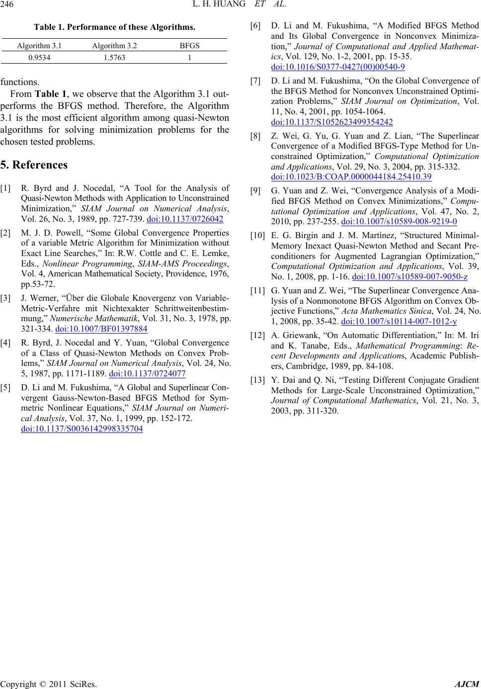 L. H. HUANG ET AL. Copyright © 2011 SciRes. AJCM 246 Table 1. Performance of these Algorithms. Algorithm 3.1 Algorithm 3.2 BFGS 0.9534 1.5763 1 functions. From Table 1, we observe that the Algorithm 3.1 out- performs the BFGS method. Therefore, the Algorithm 3.1 is the most efficient algorithm among quasi-Newton algorithms for solving minimization problems for the chosen tested problems. 5. References [1] R. Byrd and J. Nocedal, “A Tool for the Analysis of Quasi-Newton Methods with Application to Unconstrained Minimization,” SIAM Journal on Numerical Analysis, Vol. 26, No. 3, 1989, pp. 727-739. doi:10.1137/0726042 [2] M. J. D. Powell, “Some Global Convergence Properties of a variable Metric Algorithm for Minimization without Exact Line Searches,” In: R.W. Cottle and C. E. Lemke, Eds., Nonlinear Programming, SIAM-AMS Proceedings, Vol. 4, American Mathematical Society, Providence, 1976, pp.53-72. [3] J. Werner, “Über die Globale Knovergenz von Variable- Metric-Verfahre mit Nichtexakter Schrittweitenbestim- mung,” Numerische Mathematik, Vol. 31, No. 3, 1978, pp. 321-334. doi:10.1007/BF01397884 [4] R. Byrd, J. Nocedal and Y. Yuan, “Global Convergence of a Class of Quasi-Newton Methods on Convex Prob- lems,” SIAM Journal on Numerical Analysis, Vol. 24, No. 5, 1987, pp. 1171-1189. doi:10.1137/0724077 [5] D. Li and M. Fukushima, “A Global and Superlinear Con- vergent Gauss-Newton-Based BFGS Method for Sym- metric Nonlinear Equations,” SIAM Journal on Numeri- cal Analysis, Vol. 37, No. 1, 1999, pp. 152-172. doi:10.1137/S0036142998335704 [6] D. Li and M. Fukushima, “A Modified BFGS Method and Its Global Convergence in Nonconvex Minimiza- tion,” Journal of Computational and Applied Mathemat- ics, Vol. 129, No. 1-2, 2001, pp. 15-35. doi:10.1016/S0377-0427(00)00540-9 [7] D. Li and M. Fukushima, “On the Global Convergence of the BFGS Method for Nonconvex Unconstrained Optimi- zation Problems,” SIAM Journal on Optimization, Vol. 11, No. 4, 2001, pp. 1054-1064. doi:10.1137/S1052623499354242 [8] Z. Wei, G. Yu, G. Yuan and Z. Lian, “The Superlinear Convergence of a Modified BFGS-Type Method for Un- constrained Optimization,” Computational Optimization and Applications, Vol. 29, No. 3, 2004, pp. 315-332. doi:10.1023/B:COAP.0000044184.25410.39 [9] G. Yuan and Z. Wei, “Convergence Analysis of a Modi- fied BFGS Method on Convex Minimizations,” Compu- tational Optimization and Applications, Vol. 47, No. 2, 2010, pp. 237-255. doi:10.1007/s10589-008-9219-0 [10] E. G. Birgin and J. M. Martínez, “Structured Minimal- Memory Inexact Quasi-Newton Method and Secant Pre- conditioners for Augmented Lagrangian Optimization,” Computational Optimization and Applications, Vol. 39, No. 1, 2008, pp. 1-16. doi:10.1007/s10589-007-9050-z [11] G. Yuan and Z. Wei, “The Superlinear Convergence Ana- lysis of a Nonmonotone BFGS Algorithm on Convex Ob- jective Functions,” Acta Mathematics Sinica, Vol. 24, No. 1, 2008, pp. 35-42. doi:10.1007/s10114-007-1012-y [12] A. Griewank, “On Automatic Differentiation,” In: M. Iri and K. Tanabe, Eds., Mathematical Programming: Re- cent Developments and Applications, Academic Publish- ers, Cambridge, 1989, pp. 84-108. [13] Y. Dai and Q. Ni, “Testing Different Conjugate Gradient Methods for Large-Scale Unconstrained Optimization,” Journal of Computational Mathematics, Vol. 21, No. 3, 2003, pp. 311-320.
|