Technology and Investment
Vol. 3 No. 4 (2012) , Article ID: 24852 , 10 pages DOI:10.4236/ti.2012.34037
A Frontier Approach to Measuring Impact of Adoption of Flexible Manufacturing Technology on Technical Efficiency of Malaysian Manufacturing Industry
1International Graduate School of Business, University of South Australia, Adelaide, Australia
2Faculty of Management, Multimedia University, Cyberjaya, Malaysia
Email: dadol@ou.ac.lk, absade@mmu.edu.my
Received June 7, 2012; revised July 19, 2012; accepted July 26, 2012
Keywords: Flexible Manufacturing Technology; Technical Efficiency; Mass Customisation
ABSTRACT
This paper examines the impact of the adoption of Flexible Manufacturing Technology (FMT) on the Technical Efficiency of Malaysia Manufacturing Industry. Owing to the potential multicollinearity, the Principal Component Analysis has been adopted to extract the most appropriate underlying dimensions of FMT in an effort to substitute the eight FMT variables. The study has been conducted within FMT intensively adopted 16 three-digit industries that encompass 50 five-digit industries covering the years 2000-2005. The results obtained from the two situations, one, including the industry fixed effects dummy variables and the other without these, are contrasted. It is found that the model that included the industry fixed effect dummy variables possesses a greater explanatory power. The two principal components that account for the greater variation in FMT show positive and moderately significant relationship with TE. The study concludes with sufficient evidence that FMT has a direct and moderately significant relationship with TE.
1. Introduction
Over the last two decades many researchers conducted studies that examined the factors attributing to the performance of the East Asian Economies. According to Mahadevan [1] in particular, the GDP growth of these economies was found to be driven by the perspiration factor of input accumulation rather than the inspiration factor of total productivity growth (TFPG). Owing to the increasing concern regarding the continued growth of these economies, new endogenous growth theories have been adopted in an effort to explain the performance of these economies. The significance of the manufacturing sector in these economies is so much that in each economy it accounts for well over 30 percent of the overall GDP. Therefore, more focused studies looking into the inspiration factor of TFPG, which also means factor productivity should be undertaken.
According to the conventional growth accounting methodology, TFPG is considered synonymous with technological progress (TP) which is also known as technical change. According to Coelli Rao, O’Donnell and Battese [2], TP represents advances made in technology that may be represented by an upward shift in the production frontier. This methodology which is a non frontier approach, is based on the assumption that all industries are fully realising their capacity in the production process and thus, are technically efficient. In this approach, no distinction is made between TP and changes in technical efficiency (TE) with which a known technology is adopted in production. As a result, this approach does not separately account for the technological improvement embodied in labour or the capital stock (change in efficiency) contained in the TFPG. Under a newer approach named Stochastic Frontier Production Function (SFPF), originally proposed by Aigner, Lovell and Schmidt [3], output growth is decomposed into input growth and TFPG and TFPG is in turn decomposed into TP and TE. The word frontier signifies the idea of maximality and represents the “best practice” approach to production. Mahadevan [4] showed that unlike the growth accounting approach which provided a shape of an average industry, the estimation of a frontier function was heavily influenced by the best performing industries. According to Mahadevan and Kalirajan [5], TE can be due to the accumulation of knowledge in the learning-by-doing process, improvements in the instructions for mixing together raw materials, diffusion of new technology, improved managerial practices or R&D undertaken by government or profit maximising agents, or can be affected by overall market structure of industry as it affects the methods used for acquiring, developing or modifying technology.
It is widely believed that intensive regimes of contemporary manufacturing paradigms such as mass customisation, customerisation and instant customerisation can pave the way for a competitive manufacturing industry. The studies show that mass customisation is the core manufacturing paradigm. The studies also showed that the crucial determinant of the successful implementation of mass customisation is the abundant use of Flexible Manufacturing Technology (FMT) [6,7]. Kumar and Desmukh [8] remark that today’s customer not only expects quality, reliability and competitive pricing but also customised products with timely delivery, it is desirable that an organisation is as flexible as possible,. According to Sinha and Noble [9], FMT can represent a huge cost for adopting firms, but may also offer the chance to achieve competitive advantage through superior manufacturing. Therefore, it would be important to examine the causal link between the degree of FMT adoption and TE.
The average GDP growth of Malaysia during 2000- 2007 (5.5 percent) is lower than that during 1990-2000 (7.0 percent). Malaysian Manufacturing sector GDP during 2000-2007 (13.0 percent) is much lower than the same for the period 1990-2000 (4.8 percent). These are some of the key indicators to the declining competitiveness of the Malaysian manufacturing industry over the period 2000-2007. In the Malaysian manufacturing industry, FMT is widely adopted and has received the due attention from the industry policy makers. The Malaysian Industrial Development Authority (MIDA) [10] has recognised a number of promoted activities and products (for the development and production) with regard to high technology establishments. The engagement in these activities will make them entitled to pioneer status or investment tax allowance under the promotion of Investment Act 1986. This includes FMT products such as, Computer process control systems/equipment, Process instrumentation, and Robotic equipment and Computer numerical control machine tools. The Ninth Malaysia Plan which is aimed at achieving changes in the structure and improved performance of the economy with every economic sector achieving higher value added and total factor productivity. The “Thrust 1” of this Plan states that, “Application of high technology and production of higher value added products will be given emphasis. Measures will be undertaken to migrate the electrical and electronics (E&E) industry towards high-technology and higher value added activities”. Hence, the Malaysian experience is used as a case study given its suitability.
Mahadevan [1] adopted SFPF in a study on TFPG of Malaysia’s Manufacturing Industries. Sun and Kalirajan [11] found that 2.5 percent average annual rate of TP during this period was the major contributor to TFPG in the Korean manufacturing industry whereas TE grew by a modest 1.1 percent per annum. Zhang and Zhang [12] adopted SFPF to estimate the TE of China’s large and medium sized iron and steel enterprises. Lee, Kim and Heo [13] in their empirical study on TP versus TE Gains in Manufacturing Sector of Korea, adopted the nonparametric Malmquist productivity index to break down the productivity growth into two components; technological change (innovation) and efficiency change (catching up). According to Battese and Broca [14], SFPF involves an unobservable random variable associated with the technical inefficiency of production of individuals, in addition to the random error in a traditional regression model. These studies show that TE is adopted extensively to measure efficiency of the manufacturing sector.
As shown above, evidently, only a few studies have examined the impact of specific technologies on the measures of competitiveness such as productivity, technical efficiency and profitability at industry level using less aggregated data. Berndt and Morrison [15] examined the impact of high-tech investments on multifactor productivity (MFP) and three profitability measures. While the study found only limited evidence of a positive relationship between profitability and the share of high-tech capital in the total physical capital stock, it establish that they were negatively correlated with MFP. Dolage, Sade and .Elsadig [16] investigated to impact of FMT on the TFPG of Malaysian manufacturing industry and established the significance of certain types of FMT on the TFPG.
Amato and Amato [17], Dolage and Sade [18] have investigated the impact of high-tech or FMT investments on Price Cost Margin. This study established that there was a positive impact from high-tech investments regardless of whether or not the specification includes industry effects dummy variables to account for the differences in technological opportunity among industries. Hence, according to productivity literature evidently no empirical study has been undertaken to investigate the impact of FMT adoption on TE of Malaysian manufacturing industry.
2. Methodology
The basic research hypothesis of the study is:
A high degree of FMT adoption enhances TE of the manufacturing industry of Malaysia.
2.1. Estimation of TE Using SFPF
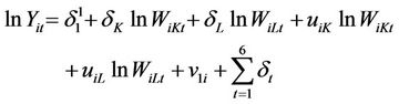
The SFPF adopted in this study to compute the industrywise technical efficiency is based on the same adopted by Mahadevan [4] in the study on “A frontier approach to measuring TFPG in Singapore Manufacturing Industry”. The derivation of the function to evaluate TE, based on SFPF is described below in Equation (1):
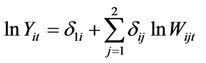 (1)
(1)
where
 (no of three-digit manufacturing industries);
j = K, and L (K-capital and L-labour);
t = 1,2,3 (no of years from 2000-2005);
Y = Value added output measured in 2000 prices;
 = Capital expenditure measured in 2000 prices;
 = Number of workers employed;
 =Intercept term of the ith three-digit manufacturing industry;
 = Actual response of output to the method of application of the jth input used by the ith manufacturing industry.
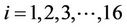
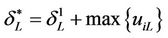
Mahadevan [19] in the study on “Is There a Real Growth Measure for Malaysia’s Manufacturing Industries?” incorporated time dummies in the SFPF to capture the effects of time on the TE. Therefore, time dummies are incorporated in this study too and accordingly Equation (1) shown above can be modified to accommodate this effect; the revised model is represented in Equation (2) shown below:
 (2)
(2)
Kalirajan and Shand [20] in their study on Frontier Production Functions and Technical Efficiency Measures, explained that the efficient use of inputs due to various industry specific characteristics contributed individually to the technical efficiency of the industry and the contributions can be measured by the magnitudes of the random slope coefficients. All other production characteristics are captured by the varying random intercept term.
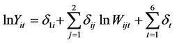
Since intercepts and slope coefficients can vary across industries they can be represented as:
 (3)
(3)
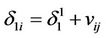 (4)
(4)
where  is the mean response coefficient of output with respect to the jth input, and
  and
and  are random disturbance terms.
Combining Equations (2), (3) and (4), SFPF can be presented in Equation (5) shown below:
 (5)
(5)
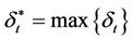
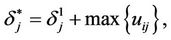
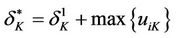
Mahadevan [21] showed that by adopting Aitken’s generalised least squares method proposed by Hildredth and Houck and the estimation procedure by Griffith the industry-specific and input-specific response coefficient estimates of the above model could be obtained. The highest values of each response coefficient and the intercept determine the frontier coefficient of the potential production function. If  denotes the parameter estimates of the frontier production function, then
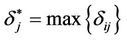 where i = 1, 2, ···16 and j = K, L
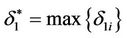 where i = 1, 2, ···16
 where t = 1, 2, ··· 6 Since
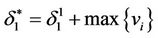
 and j represents both K and L, the above equations can be rearranged as follows:


The potential output of each industry can be realised when each industry adopts the “best practice” techniques and the maximum potential output for each industry is given by Equation (6):
 (6)
(6)
In Equation (6), since j represent both capital (K) and labour (L) it can be expanded to form a new equation (Equation (7)) which is given below:
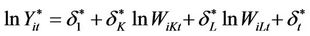 (7)
(7)
The industry-specific TE can be represented by Equation (8) shown below as the ratio of the industry’s actual realised output to that of its potential output:
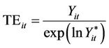 (8)
(8)
The numerator Yit can be computed simply as the “gross output” take away “cost of inputs”, values for which were obtained from ASMI.
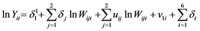
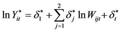
Equation (5) in which j is representative of both capital (K) and labour (L) can be expanded and presented as follows:
 (9)
(9)
All the values relating to the six years for the 50 MSIC five-digit industries (altogether 300 cases) are to be substituted in Equation (9) given above:
The technique of multiple regression analysis was adopted to ascertain the respective response coefficients for capital and labour and the constants ( ,
, ,
, and
and ). The widely used statistical software, Statistical Package for Social Sciences (SPSS) was adopted to run the above multiple regression and from its output, the maximum values for
 ,
,  and
and  were obtained to compute
 ,
,  ,
,  and
and . Once these values were ascertained, as the next step, they were substituted in the Equation (7) in order to compute the maximum frontier outputs for each industry for all the 6 years with the use of EXCEL.
2.2. Review of Factors Affecting TE in the Manufacturing Industry
Geographic Location (GLO): According to ASMI reports, Malaysia shows a significant diversity in the number of firms located within different provinces. Certain regions in a country could be disadvantaged by its distal location from the major markets due to less access to physical and human capital and technologies. Sun and Kalirajan [11] stated that firms applied their production technology and inputs differently as a result of the differences in location, experience, and firm size. Zhang and Zhang [12] stated that geographic location affected the efficiency of an enterprise. Vu [22], Margono and Sharma [23], Zhang and Zhang [12], Sun and Kalirajan [11] have considered GLO as an explanatory variable of TE.
Malaysia does not publish indicators which show the favourability of a particular province for an industry. The ASMI contains the number of establishments located within a province; usually Table 5 of ASMI depicts this information. The researcher assumes that the major reason why a large number of establishments are concentrated in a particular province is that it has a conducive environment for industries with respect to many aspects namely, access to skilled labour, technology, support industries, raw materials, close proximity to markets and ports etc. So, the corollary is that the number of firms in a province indicates the location advantage of the province. Accordingly, the provinces were ranked based on the number of establishments located in each. The directory published by Federation of Malaysian Manufacturers (FMM) contained the addresses of establishments including the province in which each establishment is situated [24]. In the FMM directory 2007, the manufacturing industries have been categorised under MSIC four-digit level. Thereafter, each establishment in a particular province was multiplied by its respective ranking. This ranking for a province was not a constant over the six year period considered since the number of establishments located within provinces has evidently changed yearly, though of course marginally. Finally, GLO was computed for each MSIC five-digit industry as the summation of the products of the number of establishment and the ranking of the respective province.
Ownership (OWN): It has long been established that generally foreign owned establishments are more efficient than locally owned establishments. Vu [22], Margono and Sharma [23], Zhang and Zhang [12], Sun and Kalirajan [11] and Mahadevan [25] considered OWN as an explanatory variable of TE. Since Malaysia is known to have a long history as a well considered recipient of FDI since mid seventies, the variable OWN was incorporated to account for the “ownership” impacts on TE.
Malaysia does not publish the status of establishments with respect to their ownership. Nevertheless, the DOS from its Economic Census data provided the number of establishments belonging to the Non Malaysian and Malaysian categories for each MSIC five-digit industry for all the years under review. Mahadevan [25] used a dummy variable “1” for industries in which more than 45 percent of the total number of establishments were either wholly foreign owned or joint ventures which were more than half foreign owned; otherwise “0”. However, information provided by the DOS in this respect was not detailed enough to assess the degree of foreign ownership regarding the Non Malaysian firms. A dummy variable (OWN) was used to distinguish between industries that had higher and lower percentages of Non-Malaysian firms. In this study, dummy variable “1” was used if in a particular five-digit industry more than 30% of the establishments were Non-Malaysian otherwise, the dummy variable “0” was used.
Firm Age (FAGE): The length of existence of a firm can indicate advancement of different factors favourable to TE namely, propensity to employ skilled workers and degree of learning by doing. According to Zhang and Zhang [12], the maturity of a firm represented by its age is a factor contributing towards inefficiency but the firm size coefficients are expected to affect inefficiency negatively. Alternatively, vintage of capital can be used to detect technical progress in production, especially the type of technical progress embodied in capital (Zhang and Zhang [12]. However, measuring the vintage of capital is not straightforward owing to the lack of data on the past capital investments at the firm level. Since it is reasonable to assume that FAGE indicates the vintage of capital and the experience of the firm, it is considered as a control variable in the TE model of this study. Sun and Kalirajan [11] as well as Margono and Sharma [23] have considered FAGE as an explanatory variable of TE in their studies.
The DOS Malaysia does not publish data pertaining to FAGE. The FMM directory gives the year of incorporation of each establishment listed under MSIC four-digit level industry. Using this value, the average FAGE for each industry was computed as at year 2000. The average firm age (FAGE) for the later years was computed by increasing the average firm age as of 2000 by one for each subsequent year.
Incentive Payments (INC): It is rational to consider that incentive schemes and bonus payments can motivate employees to work hard resulting in efficiency gains for the industry. Mahadevan [25] highlights differential incentive systems as one of the factors causing inefficiency. However, in this study INC has not been incorporated in the TE model as an explanatory variable. Vu [22] has included bonus payments as one of the hypothesised influencing factors in the TE model adopted to study technical efficiency of industrial state-owned enterprises. In this study, INC was measured as the ratio of incentive payment to salary. The DOS Malaysia does not publish data for INC industry-wise. The researcher computed INC from the Economic Census data maintained by the DOS Malaysia.
Firm Size (FSIZE): This variable is a crude proxy for scale of entry barrier. Theoretically, the minimum efficient plant size is a better proxy but could not be included due to the non availability of data. Higher productivity gains can be expected in the presence of oligopolistic competition. Therefore, researchers include average plant size or firm size in TE models to take account of such effects: Chandrasiri [26], Amato and Amato [17] and McGuckin [27]. However, the direction of the link is ambiguous. In two separate studies, Amato and Amato [17] and Round [28] have incorporated FSIZE in their PCM model to account for the entry barriers. In this study, FSIZE was measured as the average firm size of the eight largest firms in each industry. As these data are not annually published in Malaysia, they had to be computed using the data obtained from the Economic Census data maintained by the DOS.
The eight types of FMT considered in this study are given below:
Computer Numerical Control Machine Tools (CNC): Measured as the percentage of firms in each MSIC fivedigit industry using microprocessor based numerical control technologies, referred to as computer numerical control machine tools.
Numerical Controlled Machine Tools (NC): Measured as the percentage of firms in each MSIC five-digit industry using numerical controlled machine tools.
Robotics (ROB) Measured as the percentage of firms in each MSIC five-digit industry using robotics.
Programmable Logic Controllers (PLC): Measured as the percentage of firms in each MSIC five-digit industry using programmable logic controllers.
Automated Inspections (INS): Measured as the percentage of firms in each MSIC five-digit industry using automated sensor-based inspection, either during the production process or final product.
Automated Storage and Retrieval Systems (ASR): Measured as the percentage of firms in each MSIC fivedigit industry using automated storage and retrieval systems.
Computer Aided Design (CAD): Measured as the percentage of firms in each MSIC fivedigit industry using computer aided design to control manufacturing machinery.
Local Area Networks (LAN): Measured as the percentage of firms in each MSIC five-digit industry using local area networks.
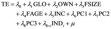
Industry Fixed Effects Dummy Variables (INDj): The study involved 50 five-digit industries included in 16 three-digit industries. It is logical to assume that industry characteristics among these 16 three-digit industries can be diverse and need to be captured by a variable. Therefore, 16 dummy variables (INDj) were incorporated into the TE model to capture the industry fixed effects. The model representing the relationship among TE explanatory variables and FMT variables can be specified as given below:
Technical Efficiency Model
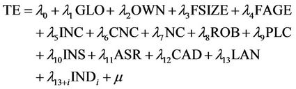 (10)
(10)
3. Data and Estimation
3.1. Inclusion Criteria
According to the Malaysian Standard Industrial Classification 2000 (MSIC 2000) there are 53 three-digit industries. In order to obtain a rational outcome, the study needs to be conducted only within industries in which FMT is intensively adopted. On account of this, inclusion criteria were formulated in an effort to select FMT intensively adopted MSIC three-digit industries for the sample, which is shown below:
Industries with high “capital/labour” ratio.
Industries in which product variation is a marketing strategy.
Industries in which products are susceptible to demand fluctuation.
Using the above criteria a sample of 16 MSIC threedigit industries which together comprise 50 five-digit industries was selected.
3.2. Primary Data
The data that indicate the degree of adoption of FMT is not published by any organisation in Malaysia. Hence, a questionnaire survey was conducted to gather information necessary to compute the percentage of establishments adopting each specific type of FMT in a given year, within a given MSIC five-digit industry. The questionnaires were sent to all the establishments, listed under the 50 MSIC five-digit industries that appeared in the directory of Federation of Malaysian Manufacturers.
3.3. Secondary Data
In order to compute TE, industry-wise data is required for output, intermediate input, capital input and labour input. The closest indicators for these values were obtained from of the ASMI published for the years 2000 through 2005 by the DOS of Malaysia. The variables GLO was computed using the data obtained from this table. OWNFISZE and INC were computed using the data obtained from the Economic Censes conducted by the DOS Malaysia. The information required to calculate FAGE was obtained from the Directory published by the Federation of Malaysian Manufacturers.
4. Empirical Results
4.1. Multicollinearity of FMT
Since only FMT intensively used industries were included in the sample, naturally some similarity in the sequence and characteristics of the production processes could be expected even amongst different five-digit industries. Hence, there could be a tendency for a similarity in the technology adopted amongst these industries. Due to the similarities in technologies, a high prevalence of multicollinearity among the eight types of FMT could be anticipated. In this study, bivariate Pearson productmoment correlation analysis has been conducted using SPSS to test for multicollinearity amongst FMT. The output that reveals potential multicollinearity among FMT variables is displayed in Table 1. According to Coakes, Steed and Price [29] and Field [30], when a considerable number of correlations are exceeding 0.3, the matrix is suitable for Principal Component Analysis (PCA).
PCA was performed using SPSS in order to obtain underlying dimensions (Principal Components) of FMT as a remedy for multicollinearity. As per both standard methods of (i.e. screen test and eigen values greater than one) extracting the optimal number of components, three Principal Components (PCs) were extracted that account for 67 percent of the variation in the FMT. According to Table 2, the loadings of variables onto the three PCs obtained from both types of rotations (Orthogonal and Oblique) are quite similar. Hence, due to simplicity, PCs obtained from orthogonal rotation was used in the rest of the analysis.
Once the most appropriate type of rotation and the resultant PCs were decided, the variables loading onto each of these PCs were examined as the next step. An examination of the component loadings depicted in Table 2 indicates that LAN, CAD, PLC and CNC load onto PC1; ASR, INS and ROB load onto PC2 while only NC loads onto PC3. Usually it is difficult to give clear cut themes or names to PCs that only relate to or encompass particular variables that are loading onto it. Hence, only the best possible names have been assigned to the PCs extracted from this analysis. The technologies LAN, CAD, PLC and CNC are used in the manufacturing set up as process control technologies. Since these load onto PC1,
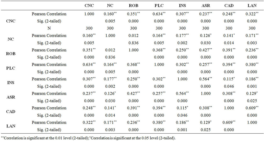
Table 1. Correlations among FMT.
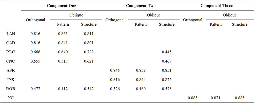
Table 2. Comparison of components obtained from two types of rotations.
so can be named as “process control” technologies. The technologies ASR, INS and ROB load onto PC2, so can be named as “production and quality control” technologies. PC3 has only one variable i.e. NC, loading onto it so can be called the “general control” technology.
As the next step, the eight FMT variables were substituted with the three PCs namely, PC1, PC2 and PC3. Therefore, the TE model was reformulated as follows:
4.2. Multiple Regression Analysis of TE
As described, the model contains a set of 16 industry fixed dummy variables (INDj) to account for the differences of technological opportunity among industries. Although it is theoretically desirable to include INDj, the consequent impact of adding these 16 extra variables needs to be examined by comparing and contrasting the results obtained without considering the INDj in the model. A separate regression was performed for this scenario and the tables of Model Summary, ANOVA and Coefficients were obtained. In order to facilitate the easy comparison of the results, the tables of output obtained from regression analysis for the two situations, one with the INDj included and the other without the INDj have been combined into one. The tables of Model Summary, ANOVA and Coefficients contained in the SPSS output for these situations have been reproduced in Tables 3-5 respectively.
According to Table 3, Adjusted R square is considerably high (0.983) when INDj has been included. This indicates that the explanatory variables together explain 51.8 percent of the variance in TE. However, the explanatory power of the model has decreased significantly when the INDj has been excluded; Adjusted R square (0.271) has decreased.
According to ANOVA, the F statistics for both situations of including and excluding INDj in the models are 10.905 and 14.884 respectively. They both are larger than the critical value (1.569) of the F distribution, obtained from the F distribution calculator for α = 0.05 level of significance when degrees of freedom are 23 and 276.
The statistical test for the existence of a linear relationship between dependent variable and the independent variables is:
As the F statistic is in the rejection region, H0 was rejected and H1 was accepted. Since “p < 0.000”, it can be concluded that there is strong evidence of TE having a linear regression relationship with any of the explanatory variables in the model with a probability of less than 0.1 percent of making an error in this conclusion.
4.3. INDj Included
According to Table 5, the variables namely, GLO (0.000) and INC (0.000) are very highly significant at “p < 0.001”. This implies that chances of making an error by assuming that these variables correlate with TE is less than 0.1 percent. Also both variables show a positive relationship with the dependent variable. FSIZE (0.136) is marginally significant at “0.10 < p < 0.15” and positively correlated whereas OWN (0.199) is insignificant and positively correlated. However, FAGE (0.889) is very highly insignificant. Since the main focus of this model is to test the
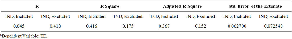
Table 3. Model summaryb.
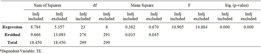
Table 4. ANOVAb.
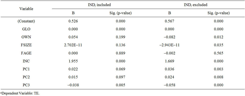
Table 5. Coefficientsa.
significance of the correlation of FMT with TE, an examination of the correlation of the three PCs with TE becomes necessary. Both PC1 (0.069) and PC2 (0.097) are moderately significant at “0.1 < p < 0.05” and positively correlated with TE. Although PC3 (0.005) is highly significant, its relationship with TE is negative.
4.4. INDj Excluded
A separate regression was performed for the scenario in which 16 INDj variables were excluded from the TE model and the tables of Model Summary, ANOVA and Coefficients contained in the respective SPSS output have been reproduced in the respective tables for the scenario of INDj excluded. The Adjusted R square (0.271) has decreased considerably. According to the output of the model that excluded the INDj, the significance of explanatory variables, GLO, OWN, FSIZE, FAGE, INCPC1, PC2 and PC3 are 0.000, 0.012, 0.035, 0.565, 0.000, 0.003, 0.008 and 0.000 respectively. One crucial difference in this model is contrary to a priori expectations, both OWN and FSIZE have negative coefficients. However, PC1 and PC2 are highly significant at “0.001 < p < 0.01” which are only moderately significant according to the model in which INDj variables were included. However, after considering all attributes it is inferred that the reliability of the first TE model which included INDj variable is higher.
For all the cases, Mahalanobis distance and Cooks distance which indicate the impact of outliers had been saved in the SPSS data editor. The critical chi-square value of 51.179 at α = 0.001 level of significance was taken as the critical value for the Mahalanobis distance. There were 19 cases which exceeded the critical value indicating that there were 19 multivariate outliers among the 300 cases. The critical value considered for the Cooks distance was one and only in two cases the critical value was exceeded.
The variables, PC1 and PC2 of the FMT which represent two important themes (dimensions), namely “process control technologies” and “production and quality control technologies” which together account for 53 percent of the variance in FMT is significant. The third PC which represents “general control technology” is insignificant and it only accounts for 13 percent of the variance in FMT. According to both TE models, the null hypotheses that PC1 and PC2 have no partial correlation with TE (i.e. λ6 = 0, and λ7 = 0) can be rejected. Moreover, the TE model which included INDj (the more reliable model), the relationship both PC1 and PC2 have with the TE is moderately significant. Therefore, the alternative hypotheses can be accepted which means that FMT has a significant correlation with TE which is positive (since in both models λ6 and λ7 are positive). This leads to the acceptance of the research hypothesis: A high degree of FMT adoption enhances TE of the Manufacturing Industry of Malaysia.
5. Conclusions
The aim of this paper was to examine the impact of the degree of adoption of FMT on the technical efficiency of the manufacturing industry of Malaysia. The types of FMT considered were namely, Computer Numerical Control machine tools (CNC), Numerical Controlled Machine Tools (NC), Robotics (ROB), Programmable Logic Controllers (PLC), Automated Inspections (INS), Automated Storage and Retrieval Systems (ASR), Computer Aided Design (CAD) and Local Area Networks (LAN). In order to remove the effects of multicollinearity among the eight types of FMT they were substituted in the regression model with the three PCs. The FMT variables load onto PCs as follows: LAN, CAD, PLC and CNC load onto PC1; ASR, INS and ROB load onto PC2 and NC only loads onto PC3. The three PCs were labelled so that they best describe their respective constituents; PC1—“process control” technologies, PC2— “production and quality control” technologies and the PC3—“general control” technology.
The most important finding of the study is that both PC1 and PC2 show moderately significant and positive relationships with TE. This indicates that the increasing adoption of process control technologies and production and quality control technologies have direct impact on TE of the FMT intensively adopted sub sector of the manufacturing industry. In contrast, PC3 shows a very highly significant and negative relationship with TE. Since both PC1 and PC2 together account for greater variation (53 percent) and PC3 account for relatively smaller variation (12 percent) among the eight FMT, it can be concluded that a high degree of FMT adoption enhances TE of the manufacturing industry of Malaysia. This is consistent with the a priori expectations regarding FMT. This shows that the degree of adoption of FMT has a positive relationship with embodied technological change which captures the effects of learning by doing (experience), advances in applied technology, managerial efficiency and industrial organisation which affords better methods and organisations that improve the efficiency of both new and old factor inputs. In other words, empirical findings of the present study postulate a correlation between the degree of FMT adoption and the above stated effects. Although the empirical findings suggest prevalence of a greater efficiency within the FMT intensively adopted industries, it does not indicate which specific effect is causing the efficiency. In the light of the deductions made in this section it can be stated that the higher the degree of adoption of FMT, the greater will be the ability to manufacture more output with the same factor inputs, in other words the ability to produce cost effectively.
In its usual call for future research, the authors recommend studies that investigate the relationship of investments in FMT rather than the degree of FMT adoption have with the TE of the manufacturing industry. It can be safely admitted that the accuracy of findings can be increased considerably by considering investments in FMT rather than the degree of adoption of FMT. Hence, it is proposed that future studies need be undertaken in collaboration with the statuary bodies established to oversee and facilitate the manufacturing industry which makes establishments obligatory to divulge investments made in FMT in order to evaluate the impact of investments in FMT on TE.
REFERENCES
- R. Mahadevan, “Perspiration versus Inspiration: Lessons from a Rapidly Developing Economy,” Journal of Asian Economics, Vol. 18, No. 2, 2007, pp. 331-347. doi:10.1016/j.asieco.2007.02.009
- T. J. Coelli, D. S. P. Rao, C. J. O’Donnell and G. E. Battese, “An Introduction to Efficiency and Productivity Analysis,” Springer, New York, 2005.
- D. J. Aigner, C. A. K. Lovell and P. J. Schmidt, “Formulation and Estimation of Stochastic Frontier Production Models,” Journal of Econometrics, Vol. 6, No. 1, 1977, pp. 21-37. doi:10.1016/0304-4076 77 90052-5
- R. Mahadevan, “A Frontier Approach to Measuring Total Factor Productivity Growth in Singapore’s Services Sector,” Journal of Economic Studies, Vol. 29, No. 1, 2002, pp. 48-58. doi:10.1108/01443580210414111
- R. Mahadevan and K. P. Kalirajan, “On Measuring Total Factor Productivity Growth in Singapore’s Manufacturing Industries,” Applied Economics Letters, Vol. 6, No. 5, 1999, pp. 295-298. doi:10.1080/135048599353267
- J. Wind and A. Rangaswamy, “Customisation: The Next Revolution in Mass Customization,” Journal of Interactive Marketing, Vol. 15, No. 1, 2001, pp. 13-31.
- G. Da Silveria and F. S. Fogliatto, “Effects of Technology Adoption on Mass Customisation Ability of Broad and Narrow Market Firms,” Gestao & Producao, Vol. 12 No. 3, 2005, pp. 347-359. doi:10.1590/S0104-530X2005000300006
- P. Kumar and S. G. Deshmukh, “A Model for Flexible Supply Chain through Flexible Manufacturing,” Global Journal of Flexible Systems Management, Vol. 7, No. 3-4, 2006, pp. 17-24.
- R. Sinha and C. H. Noble, “The Adoption of Radical Manufacturing Technologies and Firm Survival,” Strategic Management Journal, Vol. 29, No. 9, 2008, pp. 943- 962. doi:10.1002/smj.687
- Malaysian Industrial Development Authority (MIDA), “Malaysia-Investment in the Manufacturing Sector,” MIDA, 2007.
- C. Sun and K. L. Kalirajan, “Gauging the Sources of Growth of High-Tech and Low-Tech Industries: The Case of Korean Manufacturing,” Blackwell Publishing Ltd., Hoboken, 2005.
- X. Zhang and S. Zhang, “Technical Efficiency in China’s Iron and Steel Industry: Evidence from the New Census Data,” International Review of Applied Economics, Vol. 15, No. 2, 2001, pp. 199-211. doi:10.1080/02692170151137078
- J. D. Lee, T. A. Kim and E. Heo, “Technological Progress versus Efficiency Gain in Manufacturing Sectors,” Review of Development Economics, Vol. 2, No. 3, 1998, pp. 268-281. doi:10.1111/1467-9361.00041
- G. Battese and S. S. Broca, “Functional Forms of Stochastic Frontier-Production Functions and Models for Technical Inefficiency Effects: A Comparative Study for Wheat Farmers in Pakistan,” Journal of Productivity Analysis, Vol. 8, No. 4, 1997, pp. 395-414.
- E. R. Brendt and C. J. Morrsison, “High Tech Capital Formation and Economic Performance in USA Manufacturing Industries: An Exploratory Analysis,” Journal of Econometrics, Vol. 65, No. 1, 1995, pp. 9-43.
- D. A. R. Dolage, A. B. Sade and M. A. Elsadig, “The Influence of Flexible Manufacturing Technology Adoption on Productivity of Malaysian Manufacturing Industry,” Economic Modelling, Vol. 27, No. 1, 2010, pp. 395- 403. doi:10.1016/j.econmod.2009.10.005
- L. H. Amato and C. H. Amato, “The Impact of High Tech Production Techniques on Productivity and Profitability in Selected US Manufacturing Industries,” Review of Industrial Organization, Vol. 16, No. 4, 2000, pp. 327-342. doi:10.1023/A:1007800121100
- D. A. R. Dolage and A. B. Sade, “The Impact of Adoption of Flexible Manufacturing Technology on Price Cost Margin of Malaysian Manufacturing,” Technology and Investment, Vol. 3, No. 1, 2012, pp. 26-35. doi:10.4236/ti.2012.31005
- R. Mahadevan, “Is There a Real TFP Growth Measure for Malaysia’s Manufacturing Industries?” ASEAN Economic Bulletin, Vol. 19, No 2, 2002, pp. 178-190. doi:10.1355/AE19-2E
- K. P. Kalirajan and R. T. Shand, “Frontier Production Functions and Technical Efficiency Measures,” Journal of Economic Surveys, Vol. 13, No. 2, 1999, pp. 149-172. doi:10.1111/1467-6419.00080
- R. Mahadevan, “Assessing the Output and productivity Growth of Malaysia’s Manufacturing Sector,” Journal of Asian Economics, Vol. 12, No. 4, 2001, pp. 587-597. doi:10.1016/S1049-0078 01 00104-X
- Q. N. Vu, “Technical Efficiency of Industrial StateOwned Enterprises in Vietnam,” Asian Economic Journal, Vol. 17, No. 1, 2003, pp. 87-101.
- H. Margono and S. C. Sharma, “Efficiency and Productivity Analysis of Indonesian Manufacturing Industries,” Journal of Asian Economics, Vol. 17, No. 6, 2006, pp. 979-995. doi:10.1016/j.asieco.2006.09.004
- Federation of Malaysian Manufacturers (FMM), “Directory -2007,” FMM, 2007.
- R. Mahadevan, “How Technically Efficient Are Singapore’s Manufacturing Industries?” Applied Economics, Vol. 32, No. 15, 2000, pp. 2007-2014. doi:10.1080/00036840050155931
- S. Chandrasiri, “Productivity and Technology in Sri Lankan Manufacturing Industry, Human Development in a Knowledge-Based Society: Sri Lankan Scene,” The Sri Lanka Economic Association, Colombo, 2005.
- R. H. McGuckin and M. L. Streitwieser, “The Effect of Technology Use on Productivity Growth,” Centre of Economic Studies, 1996.
- D. K. Round, “Price Cost Margins in Australian Manufacturing Industries, 1971-1972,” University of Adelaide, Adelaide, 2001.
- S. J. Coakes, L. Steed and J. Price, “SPSS 15.0, Analysis without Anguish,” John Wiley & Sons Australia, Ltd., Melbourne, 2008.
- A. Field, “Discovering Statistics Using SPSS,” SAGE Publications Ltd., London, 2005.