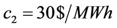
Journal of Electromagnetic Analysis and Applications
Vol. 1 No. 1 (2009) , Article ID: 196 , 13 pages DOI:10.4236/jemaa.2009.11009
Complex Dynamics Analysis for Cournot Game with Bounded Rationality in Power Market
1College of Electrical and Information Engineering, Changsha University of Science and Technology, China.
Email: yhm5218@hotmail.com
Received January 20th, 2009; revised February 11th, 2009; accepted February 23rd, 2009.
Keywords: Chaos, Dynamic Model, Nash Equilibrium, Power Market
ABSTRACT
In order to accurately simulate the game behaviors of the market participants with bounded rationality, a new dynamic Cournot game model of power market considering the constraints of transmission network is proposed in this paper. The model is represented by a discrete differential equations embedded with the maximization problem of the social benefit of market. The Nash equilibrium and its stability in a duopoly game are quantitatively analyzed. It is found that there are different Nash equilibriums with different market parameters corresponding to different operating conditions of power network, i.e., congestion and non-congestion, and even in some cases there is not Nash equilibrium at all. The market dynamic behaviors are numerically simulated, in which the periodic or chaotic behaviors are focused when the market parameters are beyond the stability region of Nash equilibrium.
1. Introduction
Some foundation industries, such as electric power, aviation, telecommunication, railroad, etc., are traditionally thought of having natural monopoly characteristics. With the development of technology, economy and society, in recent years these industries have been undergoing a market reformation tide of deregulation and competition, in order to reduce the cost and price of monopoly industry and promote the enhancement of social economy benefit. All these industries have the natural monopoly network with the complex inherent physical property, by which the market participants can provide commodity services. The complex monopoly network causes the reformation and operation of market to be more complicated and difficult than that of general commodity market, especially for the reformation of electric power industry.
In the process of reformation and operation of market, how to effectively master and supervise the dynamic market behaviors is an important research topic, especially for the power market whose reformation is carried out in its infancy stage. Taking an extreme example of California power market, the neglected study of the dynamic market behaviors led to a severe situation causing the electric power wholesale price to rise sharply and thus affecting the power supply to a lot of customers. This happened in less than three years of market operation, which has made a great impact on the economy of California and even the USA [1].
The system of market economy is essentially a dynamic system, which is mathematically represented by the differential or difference equations. In the dynamic theory of economics, there are a lot of differential or difference dynamic models, such as the classical cobweb model describing the variation of the supply and demand, the Cournot dynamic model reflecting the oligopoly market, the Haavelmo model describing the economic growth problem, and so on [2,3]. Based on these models, the analysis and control of the stable, periodic and chaotic dynamic evolution of the market economy system are investigated, and a series of results have been yielded [4,5]. However, the complex inherent physical property of network and the particularity of market transaction in the market with the monopoly network are not taken into account in these models and methods. Therefore, in view of the characteristics of power market, the research on the dynamic evolution of power market is carried out by some scholars.
The research on the dynamics of power market was first launched by F. L. Alvarado et al., via a set of one-order differential equations of power generations and consumptions. This work provides insights to the conditions for the evolving process converging to the market equilibrium, i.e., the stability condition of power market [6,7]. With the same dynamic model, a series of sufficient conditions are given to determine the stability of power market in Reference [8]. Reference [9] establishes the difference equations by taking the electricity price as a variable, and analyzes the stability condition needed for the electricity price converging to the equilibrium. Although the results achieved are interesting, these models are established based on a perfect competitive model. It neglects the game behaviors of generation companies as well as their impacts on the electricity price, and thus it can not rationally describe the actual power market.
In order to accurately simulate the game behaviors of the market participants, the oligopolistic game models in economics are further introduced to research the dynamics of power market. References [10,11] adopt the Cournot model to establish the differential equations of the dynamic power market. Then, the market equilibrium of the generation quantities is calculated under the given demand function, and the varying curve of electricity price converging to the equilibrium is numerically simulated. In References [12,13], the dynamic differential or difference equations are established based on the perfect competitive model, the Stackelberg game model and the Cournot game model, respectively. However, the constraints of power network and their impacts on the electricity price are not taken into account, nor are the stability analysis of the market equilibrium involved. In Reference [14], the evolutionary game is introduced to establish the dynamic evolutionary differential equations by taking the generation bids as variables. However, the constraints of power network are not taken into account, too.
Consequently, not only the rational game behaviors of market participants but also the inherent physical properties of power network need to be considered in the dynamic modeling of power market. In addition, due to the complex dynamic characteristics of the actual power market, in some cases there exists no market equilibrium at all, or even if there is, it might lie in the non-stability region of the market equilibrium. It is significant for the market operators to study the dynamic behaviors of the power market associated with these cases.
Therefore, the aim of this paper is to make a thorough study concerning the dynamic Cournot game behaviors of the power market with bounded rationality under the consideration of the power network constraints. The following aspects are focused:
1) A new dynamic Cournot game model of power market, represented by the difference equations embedded with the maximization problem, is proposed. The remarkable characteristic of the model is twofold: it adopts a dynamic adjustment where the limit point is the Nash equilibrium of power market; and the system of discrete difference equations embedded with the maximization problem considers the constraints of power network.
2) The existence and stability of Nash equilibrium for a duopoly game are quantitatively analyzed with different market parameters under different operating conditions of power network;
3) The dynamic behaviors of power market, especially the periodic and chaotic dynamic behaviors when the market parameters are beyond the stability region of equilibrium, are numerically simulated.
2. Dynamic Cournot Game Model of Power Market with Bounded Rationality Considering Network Constraints
2.1 Dynamic Cournot Game Model with Bounded Rationality
Power market is different from general competitive commodity market, in which the production of power energy needs very high cost and technology, and there are finite electric power producers. This nature of electric power industry implies that power market does not have the characteristic of perfect competitive market, but should belong to an oligopolistic market. In economics, several kinds of game models have been proposed to simulate the oligopolistic behaviors of market participants. The Cournot game model is most commonly used which simulates the competition of output quantities between the oligopolists [15].
Recently, the static Cournot models are applied to analyze the Nash equilibrium of power market [16,17]. In this case, the game of market participants is done based on a fully rationality. Each participant has complete market information (including the competitors’ profit functions) when he makes his optimal production decision. If there is a Nash equilibrium in the market, the oligopolists can move straight (in one shot) to the Nash equilibrium. The process is independent of the initial condition and does not relate to any dynamic adjustment of power market.
However, in the actual power market, the market participants are not fully rational and unable to know the competitors’ production decision and profit functions. They are unable to reach the equilibrium condition at once. In fact, each participant is bounded rational and can only decide the production strategy according to his expected marginal profit at each period. For each market participant, the evaluation of his own marginal profit is more accurate than the prediction of the competitors’ outputs [18,19]. Therefore, the market participants play a Cournot game with bounded rationality in a dynamic adjustment process described as follows.
In the market operation, a generation producer decides the optimal production strategy according to its own generation cost and market information in order to obtain maximum profit. The optimal decision problem can be mathematically written as
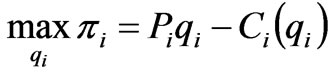 (1)
(1)
where 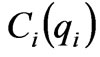 is the generation cost of generation company at node
 ;
;  is the electricity price at node
 , which is decided by the Independent System Operator (ISO). By applying the marginal profit function of a generation company, the optimal generation quantities can be obtained.
 (2)
(2)
Due to the lack of global information of power market, each generation company adjusts its supply quantities for obtaining more benefit according to the local estimate of its own marginal profit. The mathematical model of the adjustment mechanism of the generation quantities, i.e., the dynamic Cournot game model with bounded rationality is
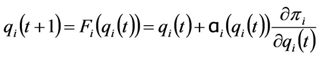
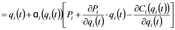
 (3)
(3)
where ,
,  are the generation quantities of the generation company at node
  at time
  and
and ;
;  is a positive function which gives the extent of the production variation of the
  generation company following a given profit signal. If
  is assumed to be a linear function, then
  can be obtained, where the positive constant
  is called the speed of adjustment.
From (3) it can be seen that in order to cause the generation company to obtain a more economical profit in the power market, if its marginal profit is greater than 0, the generation company will increase  in the next time; otherwise, the generation company will decrease
  in the next time.
2.2 ISO Optimization Model
In the power market, the decision behaviors of market participants should be checked by the ISO to satisfy the inherent physical characteristics of power network and ensure the security of power system operation. In the centralized market clearing, on the premise that the supply quantities of the generation companies are known (which can be determined by the dynamic Cournot game model of the market participants in (3)), the ISO allocates the market demand to maximize the total market benefit with satisfying the power network constraints, such as the power balance constraint and the line flow constraints. The mathematical model based on the DC power flow can be expressed as follows:
 (4)
(4)

where N is the total number of nodes ( where node N is assumed to be the slack node), L is the total number of lines;  are the nodal demand and generation power vectors excluding the slack node N,
  are the demand and generation power at the slack node N;
  denotes the transfer admittance matrix that represents the sensitivity of the nodal power injection to line power flow;
  is a vector of all ones;
  is the vector of maximum power flow on the transmission line;
  is the vector of the nodal benefit of consumer excluding the slack node N,
  is the benefit of consumer at the slack node N, and assumed as
 (5)
(5)
where  are the linear and quadratic coefficients of the consumer benefit function.
The Lagrange function for the optimization problem in (4) can be set up (in the constraints of line power flow, only the equality constraints are taken into account):
 (6)
(6)
where  are the Lagrange multipliers for the power balance constraint and the line flow constraints;
  are the matrices
  excluding the terms corresponding to the non-congestion lines.
By , the function relationship between the electricity price and the generation quantities can be obtained as follows:
1) When the congestion occurs in the power network,
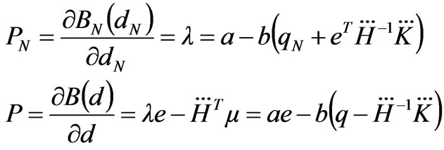 (7)
(7)
2) When the congestion does not occur in the power network,
 (8)
(8)
where  is the nodal price vector excluding the slack node N,
  is the nodal price at the slack node N.
From (7) and (8), it can be concluded that when there is no congestion in the power network, all nodal prices are identical; while during congestion, the nodal prices are different and related to the congestion conditions of power network. With the change of congested lines, the matrices  is varied, and then the function relationship between the nodal price and generation quantities is changed.
A further analysis is performed with an example of simple power market as shown in Figure 1. There are two zonal markets connected by a transmission line with capacity . The electricity prices of the two zonal markets are
 , with the demand quantities being
  and the generation quantities as
 .
.
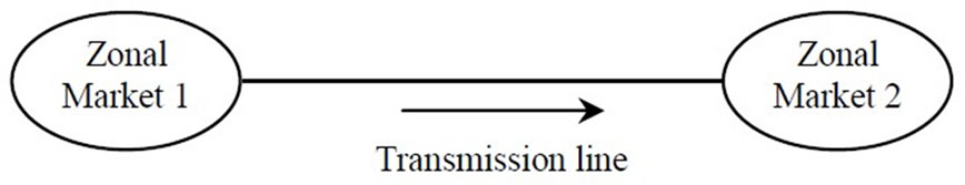
Figure 1. Structure of power market
For simplicity, the benefit of consumers is identical in these two zonal markets. In the calculation, suppose node 2 is the slack node, the positive direction of line power flow denoted by the arrow in Figure 1.
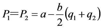
By establishing the optimization model in (6), the function relation between the zonal prices and the generation quantities are deduced from (7) and (8). When the transmission line is not congested, the zonal prices are
 (9)
(9)
In this case, the power flow on the transmission line satisfies:
i.e.,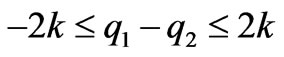 .
.
When the transmission line is congested and its power flow is , the zonal prices are
 (10)
(10)
Similarly, when the line power flow is , the zonal prices are
 (11)
(11)
Therefore, under the consideration of power network constraints, the price function of power market exhibits the following piecewise form:
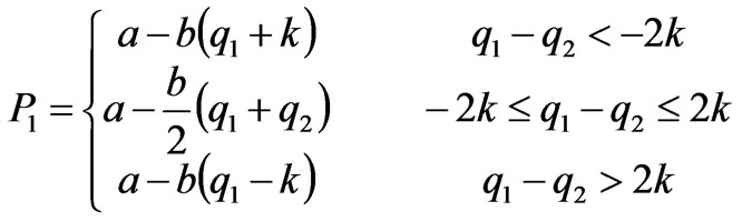 (12)
(12)
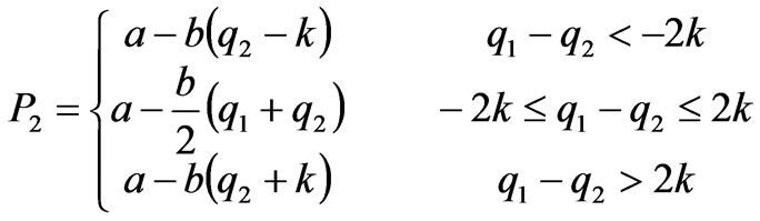 (13)
(13)
Figure 2 shows the piecewise continuous curve of electricity price function in the zonal market 1.
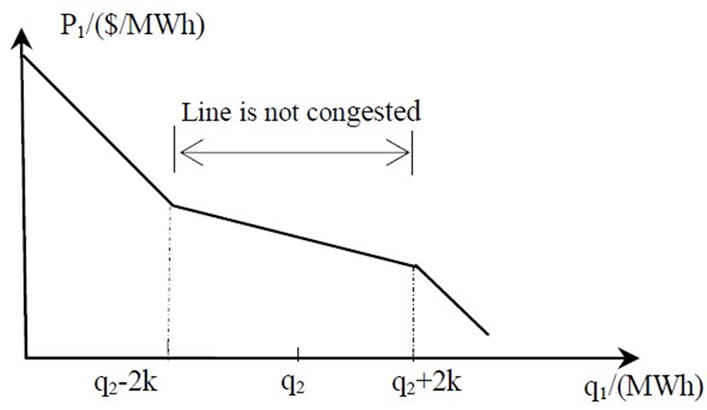
Figure 2. Curve of electricity price of zonal market 1
2.3 Dynamic Model of Power Market
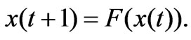
The dynamic model of power market is an integration of the dynamic Cournot game model with bounded rationality, i.e., the discrete difference equations in (3), and the maximization model of market benefit considering the power network constraints, i.e., the optimization model in (4). Therefore, the dynamic model of power market is represented by the discrete difference equations embedded with the optimization problem. Compared with the existing dynamic models, the remarkable characteristics of the proposed one are 1) The market participants need not have global market information, such as the market demand and the competitors’ cost. They decide their generation quantities by estimating their own marginal profit. This decision process reflects the actual situation of the economic system to a certain extent, indicating some feasible and rational features.
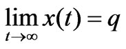
2) If the dynamic system is finally able to converge to the equilibrium condition, i.e. , each generation company reaches its own maximum profit and is unable to improve the profit only by changing its own generation strategies. In this situation, the market reaches the condition of Nash equilibrium.
3)  is the marginal profit function. From (3), it can be observed that if
 , the generation company will increase
  in the next time; otherwise, the generation company will decrease
 .
.
4) The system of discrete difference equations embedded with the optimization problem considers the impact of the power network constraints on the behaviors of the market participants. It can indicate that the dynamic model of power market is more complex than that of general commodity market.
For a duopoly Cournot game as shown in Figure 1, the dynamic Cournot model of power market with bounded rationality considering the power network constraints is

if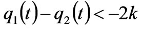 (14)
(14)
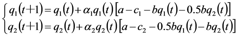
if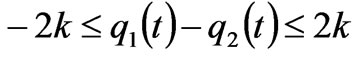 (15)
(15)
if (16)
(16)
3. Nash Equilibrium and Local Stability of Power Market
3.1 Nash Equilibrium of Power Market
Definition 1: A Nash equilibrium for (1) is a vector  such that for each participant
 , given all other participants’ output
 ,
,  maximizes the
  participant’s profit, that is
 .
.
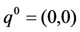
In the dynamic model (3), if , the market arrives at a fixed point. It is called the equilibrium point in economics, where the fixed point
  is the boundary equilibrium point. It is easy to verify that the nonzero fixed point is the Nash equilibrium point.
For the duopoly dynamic game in the simple power market as shown in Figure 1, represented by (14), (15), (16), the equilibrium points of the market are analyzed under the different operating conditions of power network, i.e., congestion or non-congestion. In the model, suppose the generation cost function is in linear form, i.e.,
 (17)
(17)
where  are the marginal generation costs.
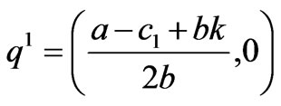
If ≤
≤ ≤
≤ , the transmission line is not congested. By solving the fixed points in (15), we can have at most 4 equilibrium points:
 ,
, ,
,  ,
,

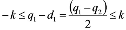
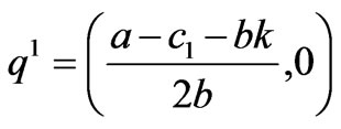
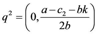
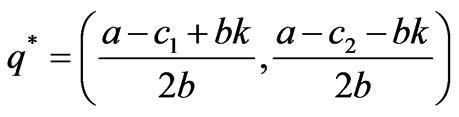
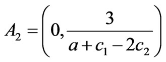
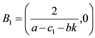
where  are the boundary equilibriums, and
  is the Nash equilibrium. Due to the satisfaction of the conditions -2k≤q1-q2≤2k, q1, q2≥0, only the equilibrium points q1, q2 and
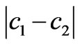
  are effective if 0<a-c1≤2bk, 0<a-c2≤2bk, a+c2-2c1≥0, a+c1-2c1≥0, -bk<c1-c2≥bk.
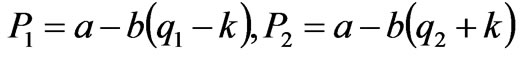
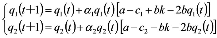
If q1-q2<-2k or q1-q2<2k, the transmission line is congested. By solving the fixed points in (14), we can have at most 4 equilibrium points:
 ,
,  ,
,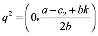 ,
,

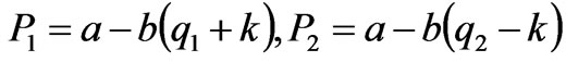
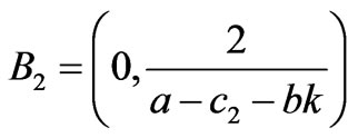
Due to the satisfaction of the conditions q1-q2<-2k, q1,q2≥0, only the equilibrium points q2 and q* are effective if a-c1>bk, c1-c2>2bk. By solving the fixed points in (16), we can have at most 4 equilibrium points:
 ,
,  ,
,  ,
,
Due to the satisfaction of the conditions q1-q2>2k, q1,q2≥0, only the equilibrium points q1 and q* are effective if a-c2>bk, c2-c1>2bk.
From the above analysis, it is found that there are different Nash equilibriums in the power market under different operational conditions of power network, such as congestion and non-congestion, while in some cases there is no Nash equilibrium at all if the market parameters satisfy <
< <
< .
.
3.2 Local Stability of Nash Equilibrium
The local stability of equilibrium point is studied based on the complex plane of the eigenvalues of the Jacobian matrix of the mapping
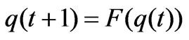
Definition 2: For a dynamic system
 , with a fixed point q, if all the eigenvalues of the Jacobian matrix
  is less than 1 in modulus, there exists an open neighbourhood I of q. When
 , such that
here, q is called the local stable fixed point [20].
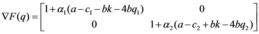
If ≤q1-q2≤2k, the transmission line is not congested, the Jacobian matrix
 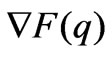 is denoted as
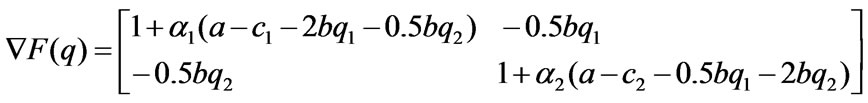
when the market lies in the Nash equilibrium point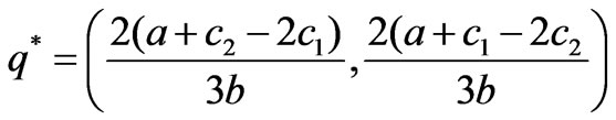 , the eigenvalue equation of the Jacobian matrix
  is:
is:
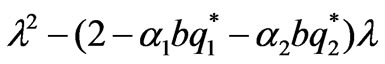

The stability condition of Nash equilibrium point is <1,
<1, <1, and thus the market parameters should satisfy:
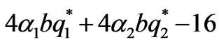 <
< <0(18)
when the market equilibrium point is , the two eigenvalues of the Jacobian matrix
  are
are
 <1
<1
 >1 Thus, the boundary equilibrium point
  is unstable. Similarly, it is easy to prove that the boundary equilibrium point
  is unstable too.
If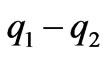 <-2k, the transmission line is congested, the Jacobian matrix
  is denoted as
when the market lies in the Nash equilibrium point , the stability condition of Nash equilibrium point is:
 <1,
<1, <1(19)
when the market equilibrium point is , one of the eigenvalues of the Jacobian matrix
  is greater than 1. Thus, the boundary equilibrium point
  is unstable.
If q1-q2>2k, it is easy to prove similarly that the boundary equilibrium point q1 is unstable, and while the Nash equilibrium point q* is stable if <1,
<1, <1.
<1.
Therefore, in the dynamic Cournot game, whether the market can finally converge to a certain Nash equilibrium point is decided by the market parameters and the line flow limits, i.e.1) When the difference between the marginal cost of generation companies is less than , i.e.,
 <c1-c2<bk (the other market parameters satisfy
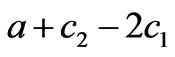 ≥0,
≥0,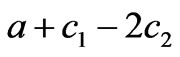 ≥0) and the market parameters satisfy the condition in (18), the generation quantities of generation companies do not greatly differ in different zonal markets. Thus, the transmission line can not be congested. In this situation, if the generation quantities fall inside the stability region of Nash equilibrium, the market will be able to gradually converge to the Nash equilibrium point q*
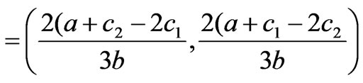 (20)
(20)
2) When the difference between the marginal cost of generation companies is greater than 2bk, i.e.,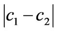 >2bk (the other market parameters satisfy a-c1>bk or a-c2>bk) and the market parameters satisfy the condition in (19), the generation quantities of generation companies greatly differ in different zonal markets. Thus, the transmission line is congested. In this situation, if the generation quantities fall inside the stability region of Nash equilibrium, the market will be able to gradually converge to the Nash equilibrium point q*
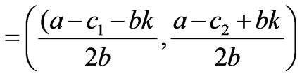
or q*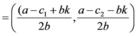 (21)
(21)
3.3 Effect of Market Parameters on Stability
The equation in (18) gives the stability condition of Nash equilibrium if the line is not congested. Figure 3 shows the corresponding stability region of Nash equilibrium point in the plane of the adjustment speeds , which is bounded by the portion of hyperbola, i.e.,

where:
 ,
, (22)
(22)
For the values  inside the stability region, the Nash equilibrium is stable. From Figure 3, the increment of the adjustment speeds will reduce the stability margin when the other parameters are fixed. If the adjustment speeds go beyond the stability region, the Nash equilibrium point loses its stability through a period-doubling bifurcation.
If the parameter , the maximum electricity price of electric power, is increased and the other parameters
 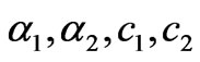 are fixed, the stability region becomes smaller, as can be easily deduced from (22). Otherwise, if the parameter
  is reduced, the stability of Nash equilibrium can be reinforced.
If the other parameters are fixed, an increment of the marginal generation cost  causes a displacement of the point
  to the right and of
  downwards. Instead, an increment of the marginal generation cost
  causes a displacement of the point
  to the left and of
  upwards. In both cases, the effect on the stability of Nash equilibrium point depends on the position of the point
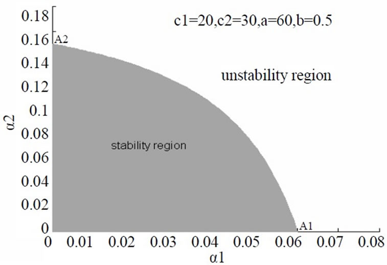
Figure 3. Stability region of Nash equilibrium under noncongestion
Figure 4. Stability region of Nash equilibrium under congestion
 . In fact, if the point
  is above the diagonal
 , i.e.,
  , an increment of
  can destabilize the Nash equilibrium point, whereas an increase of
  reinforces its stability. The situation is reversed if
 .
.
The equation in (19) gives the stability condition of Nash equilibrium if the line is congested. Figure 4 shows the corresponding stability region of Nash equilibrium point in the plane of the adjustment speeds .
.
where:
 ,
,
if 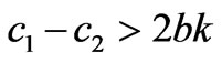
or 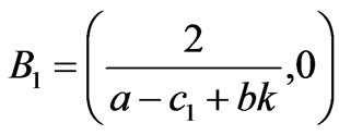 ,
,
if  (23)
(23)
From Figure 4, the increment of the adjustment speeds  and the maximum price
  can cause a loss of stability of Nash equilibrium, and while the increment of the marginal cost
  and
and  can reinforce its stability.
Therefore, the power market can be kept in the stable equilibrium condition by the following measures in the actual operation.
1) The plentiful competition is introduced to reduce the difference between the generation marginal cost of generation companies in the power market; and the rational power network planning can improve the transfer capacity of lines, in order to keep the market in the stable equilibrium.
2) The variation extent of the generation quantities is not too large; and the smooth operation of the generator has important effect not only on the stability of power system but on the stability of power market.
3) The maximum price of market is not too high; and the restriction of the maximum value of electricity price can reinforce the stability of power market.
4. Numerical Simulation of Dynamic Market Behaviors
The dynamic behaviors of power market are demonstrated with an example of two-node power market as shown in Figure 1. The evolving characteristics of market behaviors are analyzed when the parameters lie in different ranges by using the bifurcation diagram, phase diagram, Lyapunov exponent and fractal dimension. In the iterative process of the numerical simulation, the benefit of consumers is identical and assumed with  and
and
 ; the maximum production outputs of the two generation companies both are 200MWh; the flow limits of the line is 30MW.
4.1 Case 1: Difference between Marginal Cost of Generation Companies is Less than bk
Firstly, the dynamic behaviors of power market are numerically simulated when the difference between the marginal cost of the two generation companies is less than , i.e.,
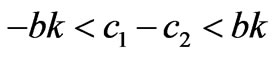 . The generation marginal costs are taken as
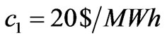 ,
, . If different values are selected, similar results can be obtained. In this case, a Nash equilibrium point is obtained. By (20), the corresponding generation quantities of the two zones are (66.67MWh, 26.67MWh).
Let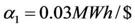 , the adjustment speed of the generation quantities of generation company 2 is changed. Figure 5 shows the bifurcation diagram of the stable solutions of the generation quantities and electricity price with
 . When the adjustment speed of generation company 1 is changed, similar results can be obtained.
If the adjustment speed of the generation quantities of generation company 2 satisfies <0.12, the market lie in the stability region of Nash equilibrium. The generation quantities will gradually converge to the unique stable solution, i.e., the Nash equilibrium point (66.67MWh, 26.67MWh). In this case, the power flow on the line is 20MW, that is, the line is not congested. Thus, the electricity price of the two zones is identical, both being 36.67$/MWh. Figure 6 shows the evolving curve of the market converging to the Nash equilibrium if
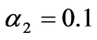 .
.
With the increment of the adjustment speed , when
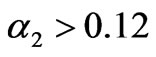 , the market will go beyond the stability region of Nash equilibrium and thus loses stability. If
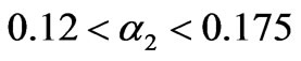 , the dynamic evolution of the generation quantities and electricity price will converge to the two periodic points and the two-period variation is exhibited. Sequentially, with the increment of
 , the more complex dynamic behaviors are exhibited, such as four periods, eight periods, sixteen periods, etc. Figure 7 shows the periodic evolving curve of the market if
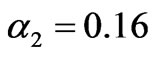 .
.
With the continuous increment of the adjustment speed , when
 , the market converges to many infinite points inside the bounded range and the seemingly random chaotic variation is exhibited. When
  is in the neighborhood of 0.18, the stable solutions of the market lie within a smaller range. In this case, the power flow on the line is less than 30MW, that is, the line is not congested. Thus, the electricity price of zonal market 1 and 2 is identical. Figure 8 shows the chaotic evolving curve of the generation quantities and electricity price if
 ; and the corresponding chaotic attractors as shown in Figure 9.
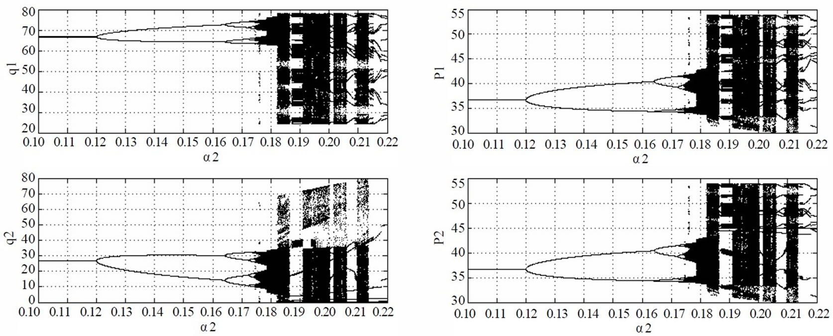
Figure 5. Bifurcation diagram of stable solutions of power market with α2 if difference between marginal cost of generation companies is less than bk
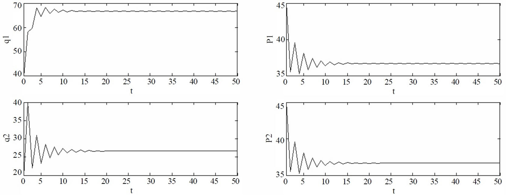
Figure 6. Dynamic market behaviors converging to Nash equilibrium if α2=0.1

Figure 7. Periodic dynamic market behaviors if α2=0.16
However, when the adjustment speed  lies in the other chaos area, the stable solutions of the market fall within a greater range. In this case, it is found that the line sometimes is congested to cause different electricity price in the zonal market 1 and 2; the chaotic attractors of market include not only the invariable manifold under non-congestion condition (as shown in Figure 9), but the invariable manifold under congestion condition. Figure 10 shows the chaotic attractors of the generation quantities and electricity price if
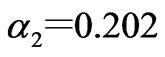 , their maximum Lyapunov exponents and fractal dimensions being 0.34 and 1.10, respectively.

Figure 8. Chaotic dynamic market behaviors if α2=0.18

Figure 9. Chaotic attractors of generation quantities and electricity price if α2=0.18
Figure 10. Chaotic attractors of generation quantities and electricity price if α2=0.22
4.2 Case 2: Difference between Marginal Cost of Generation Companies is Greater than 2bk
The dynamic behaviors of the power market are numerically simulated when the difference between the marginal cost of the generation companies is greater than , i.e.,
 . The generation marginal costs are taken as
 ,
,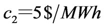 . If different values are selected, similar results can be obtained. In this case, a Nash equilibrium point is obtained. By (21), the corresponding generation quantities of the two zones are (5MWh, 70MWh).
Let , the adjustment speed of the generation quantities of generation company 2 is changed. Figure 11 shows the bifurcation diagram of the stable solutions of the generation quantities and electricity price with
 . When the adjustment speed of generation company 1 is changed, similar results can be obtained.
If the adjustment speed of the generation quantities of generation company 2 satisfies , the market lie in the stability region of Nash equilibrium. The generation quantities will gradually converge to the unique stable solution, i.e., the Nash equilibrium point (5MWh, 70MWh). In this case, the power flow on the line is 30MW, that is, the line is congested. Thus, the electricity price of the two zonal markets is not identical, being 42.5$/MWh and 40$/MWh, respectively.
With the increment of the adjustment speed , when
 , the market will go beyond the stability region of Nash equilibrium and thus loses stability. The dynamic market behaviors exhibit the periodic and chaotic variation. The constraint of transmission line change the route of period-doubling bifurcation to chaos, exhibiting intermittency. Figure 12 shows the chaotic evolving behaviors if
 . The corresponding chaotic attractors are shown in Figure 13, their maximum Lyapunov exponents and fractal dimensions being 0.53 and 0.60.
Figure 11. Bifurcation diagram of stable solutions of power market with α2=0.22 if difference between marginal cost of generation companies is greater than 2bk
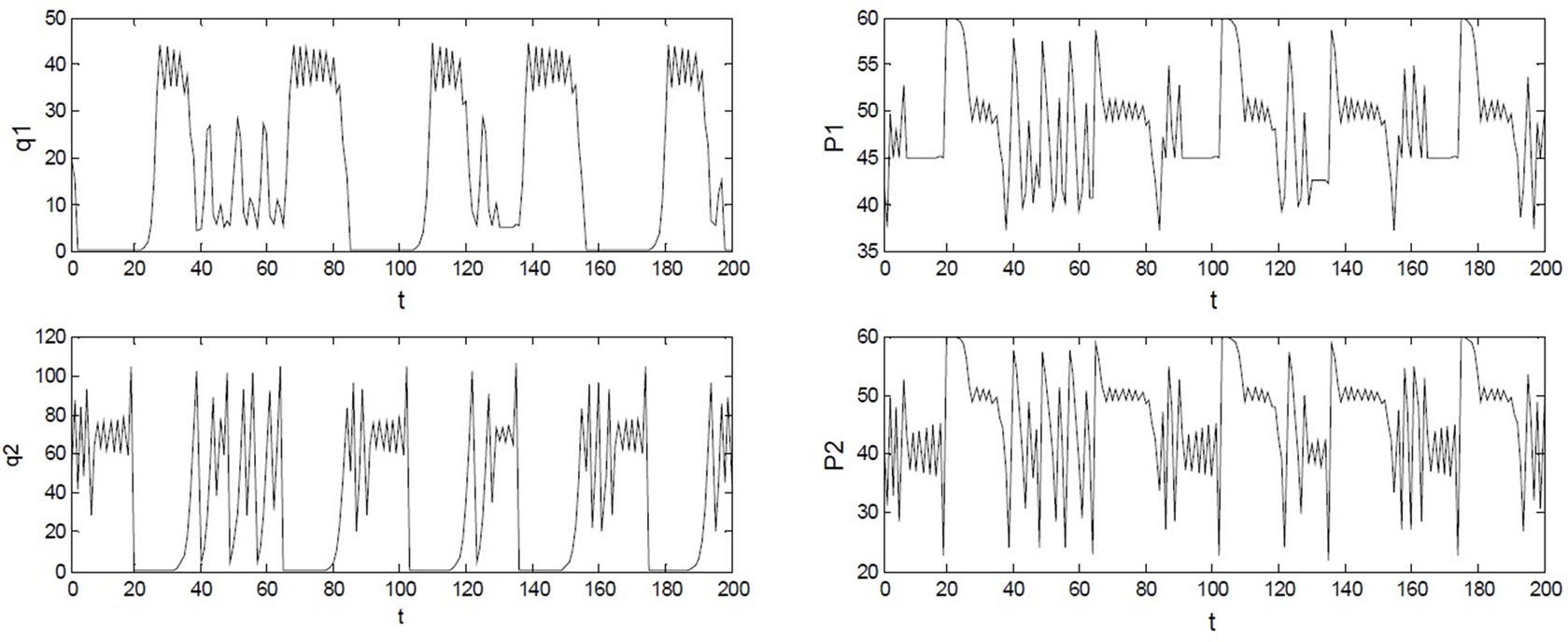
Figure 12. Chaotic dynamic market behaviors if α2=0.03

Figure 13. Chaotic attractors of generation quantities and electricity price if α2=0.03
4.3 Case 3: Difference between Marginal Cost of Generation Companies Lies in [bk, 2bk]
The dynamic behaviors of the power market are numerically simulated when the difference between the marginal cost of the generation companies lies in , i.e.,
 . The generation marginal costs are taken as
 ,
, . Similar results can be obtained for other selected values. By the analysis of Section 3.1, there is no Nash equilibrium point in this case, that is, no matter how large the adjustment speeds are, the market cannot converge to a stable Nash equilibrium at all. Figure 14 shows the bifurcation diagram of the stable solutions of the generation quantities and electricity price with
  (where
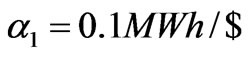 ).
).
From Figure 14, it is found that the dynamic market behaviors exhibit the periodic and chaotic variation; and the chaotic and periodic windows appear in turn. Figure 15 shows the chaotic attractors of the generation quantities and electricity price if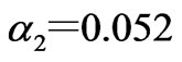 , their maximum Lyapunov exponents and fractal dimensions being 0.23 and 0.80, respectively.
Whether the transmission lines is congested or not, if the market participants with bounded rationality continuously adjust their production strategies, the market will finally converge to the Nash equilibrium under the satisfaction of its stability condition. Sequentially, a state that the market participants simultaneously maximize their respective profit is achieved.
In the complex dynamic power market, the equilibrium condition is short-term and temporary. In the equilibrium condition, many uncertain factors, such as the adjustment speeds and marginal cost of generation companies, the maximum electricity price of market, are changing the operating condition of market and pushing it towards chaos. The appearance of market chaos is very sensitive to the market parameters. The change of parameters can lead to a great difference between the long-term evolving trajectories of the dynamic market. Once the market enters the chaotic condition, it will be unpredictable, in which the generation companies are unable to effectively determine the adjustment of output quantities in the long term.
Figure 14. Bifurcation diagram of stable solutions of power market with α2 if difference between marginal cost of generation companies lies in [bk,2bk]
Figure 15. Chaotic attractors of generation quantities and electricity price if α2=0.052
However, when the market lies in the chaotic condition, it is still possible to effectively predict the short-term dynamics and change the chaotic market attractors to control the chaos. Therefore, in the case, the generation companies with bounded rationality should continuously survey their own surroundings and adjust their operation objectives. The market managers should timely modify the operation rules in order to change the chaotic market attractors and adapt the variation of the market environment.
5. Conclusions
This paper proposes the dynamic Cournot game model with bounded rationality considering the power network constraints, i.e., the difference equations embedded with the optimization problem. By using the theory of nonlinear discrete dynamic system, the Nash equilibrium and its stability for a duopoly market are quantitatively analyzed. It is found that the power market has different Nash equilibriums with different market parameters corresponding to different operating conditions, i.e., congestion and non-congestion, while in some cases it has no Nash equilibrium at all. The effect of market parameters is investigated on the stability of Nash equilibrium. It is also revealed that the smooth adjustment of the generation quantities and the restriction of the maximum value of electricity price can reinforce the stability of the power market. In the dynamic evolution, the market exhibits a variety of dynamic behaviors, i.e., converging to the Nash equilibrium, period and chaos.
Based on the above work, there are the following issues need to be explained and discussed.
(a) For descriptive simplicity, the generation marginal cost is assumed to be a linear form in this paper. If it is a quadratic function, the Nash equilibriums of market and their stability conditions may be similarly obtained, as well as the periodic and even chaotic dynamic behaviors when the market go beyond the stability region.
(b) In the dynamic Cournot game, the generation quantities are regarded as the decision variables of generation companies, which may be sold to the users through the contract transaction, also to the Power Exchange through the Pool transaction. So long as the relationship between the demand and electricity price is identical in the two transaction models, the similar results, such as the same market equilibrium points and dynamic behaviors, can be obtained.
6. Acknowledgements
This work is supported by the National Natural Science Foundation of China (No.70601003) and the Program for New Century Excellent Talents in University of China.
REFERENCES
- W. W. Hogan, “California market design breakthrough,” Harvard University, Cambridge, 2002.
- D. X. Zhang and Z. H. Chen, “Nonlinear dynamic economics-bifurcation and chaos,” Ocean University Press of Qingdao, Qingdao, 1995.
- H. N. Agiza, A. S. Hegazi, and A. A.Elsadany, “The dynamics of Bowley’s model with bounded rationality,” Chaos, Solitions and Fractals, 12, pp. 1705-1717, 2001.
- N. A. Hamdy, I. B. Gian, and K. Michael, “Multistability in a dynamic Cournot game with three oligopolists,” Mathematics and Computers in Simulation, 51, pp. 63-90, 1999.
- R. Herdrik and S. Arco, “Control of the triple chaotic attractor in a Cournot triopoly model,” Chaos, Solitions and Fractals, 29, pp. 409-413, 2004.
- F. L. Alvarado, “The stability of power system markets,” IEEE Transactions on Power Systems, 2, pp. 505-511. 1999.
- F. L. Alvarado, J. Meng, and C. L. DeMarco, “Stability analysis of interconnected power systems coupled with market dynamics,” IEEE Transactions on Power Systems, 4, pp. 605-701, 2001.
- Z. H. Yang, Y. F. Liu, and Y. Tang, ”Analysis of power market stability,” Proceedings of the Chinese Society for Electrical Engineering, 2, pp. 1-5, 2005.
- Y. D. Tang, J. J. Wu, and Y. Zou, “The research on the stability of power market,” Automation of Electric Power Systems, 4, pp. 11-16, 2001.
- A. Maiorano, Y. H. Song, M. Trovato, “Dynamics of non-collusive oligopolistic electricity markets,” IEEE Power Engineering Society Winter Meeting, Vol. 2, pp. 838-844, 2000.
- Y. B. Zhang, X. J. Luo, and J. Y. Xue, “Adaptive dynamic Cournot model of optimizing generating units’ power output under nonlinear market demand,” Proceedings of the Chinese Society for Electrical Engineering, 11, pp. 80-84, 2003.
- Y. F. Liu, Y. X. Ni, and F. F.Wu, “Control theory application in power market stability analysis,” IEEE International Conference on Electric Utility Deregulation, Restructuring and Power Technologies, Vol. 2, pp. 562-569, 2004.
- W. G. Yang and G. B. Sheble, “Modeling generation company decisions and electric market dynamics as discrete systems,” IEEE Power Engineering Society Summer Meeting, Vol. 3, pp. 1385-1391, 2002.
- J. Gao and Z. H. Sheng, “Evolutionary game theory and its application in electricity market,” Automation of Electric Power Systems, 18, pp. 18-21, 2003.
- S. Y. Xie, “Economic game theory,” 2th edition, Fudan University Press, Shanghai, 2002.
- Z. Younes and M. Ilic, “Generation strategies for gaming transmission constraints: Will the deregulated electric power market be an oligopoly?” Proceedings of the 31th Hawaii International Conference on System Sciences, Vol. 3, pp. 112-121, 1998.
- B. C. Lance, B. Ross, and L. B. Martin, “An empirical study of applied game theory: Transmission constrained Cournot behavior,” IEEE Transactions on Power Systems, 1, pp. 166-172, 2002.
- G. I. Bischi and A. Naimzada, “Global analysis of a dynamic duopoly game with bounded rationality,” Advances in Dynamic Games and Application, Vol. 5, pp. 361-385, 1999.
- H. R. Varian, “Microeconomic analysis,” 3rd edition. W. W. Norton & Company, 1992.
- A. Medio and M. Lines, “Nonlinear dynamics: A primer,” Cambridge University Press, New York, 2001.