Journal of Intelligent Learning Systems and Applications
Vol.4 No.3(2012), Article ID:22033,17 pages DOI:10.4236/jilsa.2012.43024
Regularization by Intrinsic Plasticity and Its Synergies with Recurrence for Random Projection Methods
![]()
Research Institute for Cognition and Robotics (CoR-Lab), Bielefeld University, Bielefeld, Germany.
Email: kneumann@cor-lab.uni-bielefeld.de, cemmeric@cor-lab.uni-bielefeld.de, jsteil@cor-lab.uni-bielefeld.de
Received February 22nd, 2012; revised May 23rd, 2012; accepted June 1st, 2012
Keywords: Extreme Learning Machine; Reservoir Computing; Model Selection; Feature Selection; Model Complexity; Intrinsic Plasticity; Regularization
ABSTRACT
Neural networks based on high-dimensional random feature generation have become popular under the notions extreme learning machine (ELM) and reservoir computing (RC). We provide an in-depth analysis of such networks with respect to feature selection, model complexity, and regularization. Starting from an ELM, we show how recurrent connections increase the effective complexity leading to reservoir networks. On the contrary, intrinsic plasticity (IP), a biologically inspired, unsupervised learning rule, acts as a task-specific feature regularizer, which tunes the effective model complexity. Combing both mechanisms in the framework of static reservoir computing, we achieve an excellent balance of feature complexity and regularization, which provides an impressive robustness to other model selection parameters like network size, initialization ranges, or the regularization parameter of the output learning. We demonstrate the advantages on several synthetic data as well as on benchmark tasks from the UCI repository providing practical insights how to use high-dimensional random networks for data processing.
1. Introduction
In the last decade, machine learning techniques based on random projections have attracted a lot of attention because in principle they allow for very efficient processing of large and high-dimensional data sets [1]. These approaches randomly initialize the free parameters of the feature generating part of a data processing model and restrict learning to linear methods for obtaining a suitable readout function. As opposed to random projections for dimensionality reduction, which have been considered much earlier [2,3], it is characteristic for such new approaches to use high-dimensional projections. These often actually increase the feature dimensionality.
A prominent example is the extreme learning machine (ELM) as proposed in [4]. It comprises a single hidden layer feed-forward neural network with fixed random input weights and a trainable linear output layer as depicted in Figure 1(a). ELMs have become popular, because, compared to traditional backpropagation training, they train much faster since output weights are computed in a single batch regression step. Despite this apparent simplicity, ELMs are universal function approximators with high probability under mild conditions if arbitrarily large networks can be considered [5]. The relation between the ELM approach and earlier proposed feedforward random projection methods is discussed in [6]. In practice and for a finite ELM, however, model selection, parameter initialization and regularization are challenges and active topics of research.
The most prominent other example for random projections is the reservoir computing (RC) approach [7], a paradigm to use recurrent neural networks with fixed and randomly initialized recurrent weights, see Figure 1(b). From a machine learning point of view, the reservoir serves as a fixed spatio-temporal kernel projecting the input data nonlinearly into a high dimensional space of the reservoir network states. In the limit of infinitely many neurons, this is equivalent to a recursive kernel transformation [8]. The subsequent use of a trainable
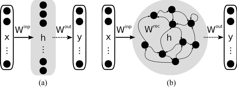
Figure 1. (a) Extreme learning machine architecture. Only the readout connections Wout are adapted during training (dashed arrows); (b) Reservoir network, comprising recurrent connections.
non-recurrent linear readout layer combines the advantages of recurrent networks with the ease, efficiency and optimality of linear regression methods. New applications for processing temporal data have been reported, for instance in speech recognition [9,10], sensori-motor robot control [11-13], detection of diseases [14,15], or flexible central pattern generators in biological modeling [16].
An intermediate approach to use dynamic reservoir encodings for processing data in static classification and regression tasks has also been considered under the notion of attractor based reservoir computing [17-19]. The rationale behind is that a recurrent network can efficiently encode static inputs in its attractors [19,20]. In this contribution, we regard static reservoir computing as a natural extension of the ELM. We point out that recurrent connections significantly enrich the set of possible features for an ELM by introducing non-linear mixtures. They thereby enhance approximation capability and performance under limited resources like a finite network size. It is noteworthy that this approach does not affect the output learning, where we will still use standard linear regression.
A central issue for all learning approaches is model selection, and it is even more severe for random projection networks because large parts of the networks remain fixed after initialization. The neuron model, the network architecture and particularly the network size strongly determine the generalization performance, compare Figure 2 upper part. In the state-of-the-art ELM approach, most of these quantities are tuned manually by means of expert knowledge about the specific task.
Several techniques to automatically adapt the network’s size to a given task have been considered [21-23], whereas success is always measured after retraining the output layer of the network. Despite these efforts, it

Figure 2. Model selection vs. feature selection.
remains a challenge to understand the interplay between model complexity, output learning, and performance: controlling the network size affects only the number of features rather than their complexity and ignores effects of regularization both in the output learning and the ratio of data points to number of neurons.
An essential mechanism to consider in this context is regularization ([24-26], Section 7 in the appendix). In this paper we distinguish two different levels of regularization: output regularization with regard to the linear output learning and input or feature regularization with regard to the feature encoding produced in the hidden layer. Output regularization typically refers to Tikhonov regularization [24] and assumes a Gaussian prior for the learning parameters. This refers to adding a term in the error function which punishes large output weights and is also known as weight decay (c.f. Section A). It is easy to implement without additional computational costs in the batch linear regression and therefore is a standard method used for both ELM [27] and reservoir computing [7,28]. A suitable Tikhonov regularization parameter must be determined by line search, which is computationally costly and performance can be undesirably sensitive to it. This is in contradiction to the original simplicity of the random projection method and we will therefore propose a method to make performance more robust with respect to the choice of the output regularization.
The designer also has to make choices with respect to the input processing, e.g. on the hyper-parameters governing the distributions of random parameter initialization, on proper pre-scaling of the input data, and on the type of non-linear functions involved.
It is therefore highly desirable to gain insight on the interaction between parameter or feature selection and output regularization. The goal is to provide constructive tools to robustly reduce the dependency of the network performance on the different parameter choices while keeping peak performance. To this aim, we investigate recurrence and intrinsic plasticity, an unsupervised biologically motivated learning rule that adjusts bias and slope of a neuron’s sigmoid activation function [29]. These are two mechanisms to influence the model’ feature complexity, which span a different axis as compared to the usual model selection approaches, see Figure 2 (horizontal axis). We analyze the complex interplay of feature and model selection by assessing properties on three levels: First, the feature complexity, i.e. the feature transformation provided by a single neuron; second, the complexity of the network function, i.e. the learned combination of features measured by its mean curvature; and third, the generalization performance. Together, these measures provide a clear picture of the advantages and disadvantages of the different models.
The remainder of the paper is organized as follows. We introduce the ELM including Tikhonov regularization in the output learning in Section 2. Then we add recurrent connections to increase feature complexity in Section 3, which results in greater capacity of the network and enhanced performance. Not unexpectedly, we observe a trade-off with respect to the risk of overfitting. In Section 4 we investigate the influence of IP pre-training on the mapping properties of ELMs and show that IP results in proper input-specific regularization. Here the trade-off is for the risk of poor approximation when regularizing too much. We proceed in Section 5 to show synergy effects between IP feature regularization and recurrence when applying the IP learning rule to recurrently enhanced ELM networks. Whereas IP simplifies the feature pool and tunes the neurons to a good regime, recurrent connections introduce nonlinear mixtures and thereby avoid to end up with a too simple feature set. We show experimentally that these two processes balance each other such that we obtain complex but IP regularized features with reduced overfitting. As a result, input-tuned reservoir networks that are less dependent on the random initialization and less sensitive to the choice of the output regularization parameter are obtained. We confirm this in experiments, where we observe constantly good performance over a wide range of network initialization and learning parameters.
2. Baseline: The Extreme Learning Machine
In 2004, Huang et al. introduced the extreme learning machine (ELM) [4], a three-layer feed-forward neural network with a high-dimensional hidden layer providing a random projection of the input through fixed random weights (see Figures 1(a) and 3). Learning is reduced to computing a simple generalized inverse by linear regression. ELMs thus train much faster than traditionally trained backpropagation networks, and even performed better on most of the tasks reported in [5]. It has also been shown in [5] that a randomly created ELM with hidden layer size R is able to perform any mapping consisting of R observations. ELMs are thus in theory universal function approximators, if permitting an arbitrary number of training samples and any hidden-layer size.
The activations of the ELM input, hidden and output neurons are denoted by x, h and y, respectively (see Figure 1(a)). The connection strengths are collected in the matrices Winp and Wout denoting the input and read-out weights. We consider parametrized activation functions
 where
where
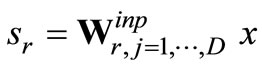
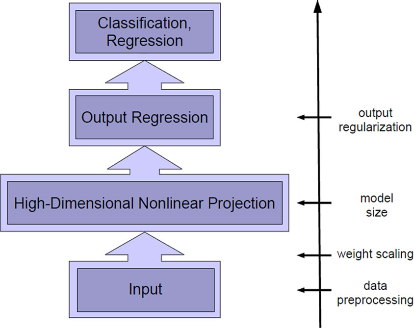
Figure 3. Machine learning view of ELMs.
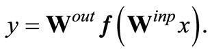
x is the total activation of each hidden neuron hr for input x and D is the input dimension. We denote ar as the slope and br as the bias of the activation function fr(·). The output y of an ELM is
 (1)
(1)
The key idea of the ELM approach is to restrict learning to the linear readout layer. All other network parameters, i.e. the input weights Winp and the activation function parameters a, b stay fixed after initialization of the network.
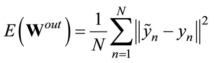
The ELM is trained on a set of training examples , n = 1, ···, Ntr by minimizing the mean squared error
 (2)
(2)
between the target outputs  and the actual network output yn with respect to the read-out weights Wout. The minimization reduces to a linear regression task given the fixed parameters and hidden activations h as follows. We collect the network’s states hn as well as the desired output targets yn in a state matrix H = (h1, ···, hNtr) and a target matrix
  for all n = 1, ···, Ntr, respectively. The minimizer is the least squares solution
 (3)
(3)
where H† is the pseudo-inverse of the matrix H.
2.1. Model Selection for the ELM
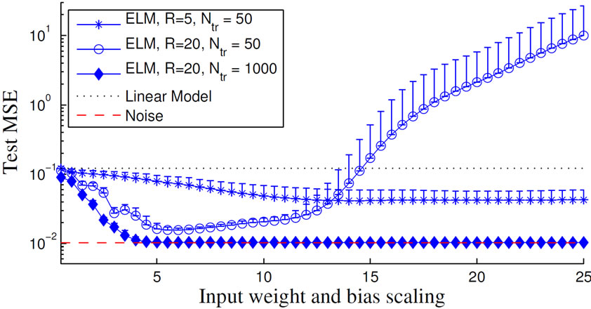
The ELM approach is appealing because of its apparently efficient and simple training procedure [5] and it has been claimed that “apart from selecting the number of hidden nodes, no other control parameters have to be manually chosen” ([30] p. 1411). However, this claim is based on the assumption that either very large data sets are used as in [5, 30, 31] or the network size is explicitly chosen to be much smaller than the number of training samples (e.g. in [12] pp. 1355-1356). In contrast, in practical applications training data can be very expensive, e.g. in tasks involving robots, and it can also be undesirable to limit the hidden layer size R to a small fraction of the number of training samples Ntr, because then the network suffers from poor approximation abilities. This is illustrated in Figure 4 (R = 5, Ntr = 50), where we show the dependency of the ELM’s generalization ability on the random distribution of the input weights Winp, the network size R and the biases b on the Mexican hat regression task (cf. Section C.2 for this often employed illustrative task). In such cases, the model selection becomes an important issue since the generalization ability is highly depending on the choice of the model’s parameters, e.g. output regularization or network size.
2.1.1. Output Regularization
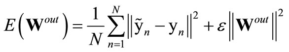
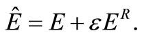
Since the ELM is based on the empirical risk minimization principle [32], it tends to over-fit the data, particularly if the task does not comprise many training samples. In the original ELM approach, over-fitting is prevented by implicit regularization: by either providing a large number of training samples (see Figure 4, R = 20, Ntr = 1000) or by using small network sizes. Assuming noise in the data, it is well known that this is equivalent to some level of output regularization [33,34]. It is therefore natural to consider output regularization directly as a more appropriate technique for arbitrary network and training data sizes as e.g. in [27,35]. As a state-of-the-art method, Tikhonov regularization ([24], Section A) can be used as in [27] which is also a standard method for reservoir networks that are introduced in Section 3. It introduces a regularization parameter ε in the error function
 (4)
(4)
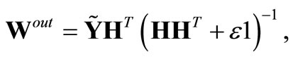
and the regularized minizer then becomes
 (5)
(5)
which is, as a side effect, also numerically more stable because of the better conditioned matrix inverse. A suitable regularization parameter ε needs to be chosen carefully. Too strong regularization, i.e. too large ε, can result in poor performance, because it limits the effective model complexity inappropriately [34]. On the other hand, a too small value of ε does not avoid the over-fitting. This is a typical model selection problem also for the ELM. The parameter ε must be determined by line search after definition of a suitable validation set, which is computationally costly.
 (a)
(a) (b)
(b)
Figure 4. (a) Development of the ELM’s average test performance; (b) Histogram of the hidden states h of one ELM for which the input weights and the biases are drawn from [–25, 25].
2.1.2. Finding the Right Initialization Ranges
In the ELM paradigm, a typical heuristics is to scale the data to [–1, 1] and to set the activation function parameters a to one [5]. Then, allowing an arbitrary large number R of hidden neurons, manual tuning of the input weights Winp or the activation function parameters a, b is not needed, because a random initialization of these parameters is sufficient to create a rich feature set. In practice, the hidden layer size is limited and the performance does indeed depend on the hyper-parameters controlling the distributions of the initialization at least of the input weights and the biases b. Very small weights result in approximately linear neurons with no contribution to the approximation capability, whereas large weights drive the neurons into saturation resulting in a binary encoding. This is illustrated in Figure 4 (R =20, Ntr = 50, where we vary the initialization range of input weights and biases b and Figure 4(b), respectively. Apparently, the choice of scaling matters.
2.1.3. The Network Size Matters
Finally, the number R of hidden neurons plays a central role and several techniques have been investigated to automatically adapt the hidden layer size. The error minimized extreme learning machine [21] and the incremental extreme learning machine [22] are methods which add random neurons to the ELM. In contrast, the optimally pruned extreme learning machine [23] pursues the idea to improve ELMs by decreasing the size of the hidden layer. All of these methods introduce considerable computational load.
In summary, the performance of the ELM on a broader range of tasks depends on a number of choices in model selection: the network size, the output regularization (or the equivalent in chosing a respective task), and the hyper-parameters for initialization. Methods to reduce sensitivity of the performance to these parameters are therefore highly desired.
3. Reservoir Networks as Natural Extension of the ELM
Adding recurrent connections to the hidden layer of an ELM converts it to a corresponding reservoir network1 (RN) (see the machine learning view on RNs in Figure 5). The RN can be used for static mapping tasks by considering the converged attractor state as encoding of the input (for more details see Section B). Then applying output regression with regularization is applied as described in the last section. In [18] and [19] this approach has been motivated by showing that for static mappings the important information is represented in the reservoir’s attractor states and in [17,19,36] it has been applied successfully. To gain insights, how and why the respective
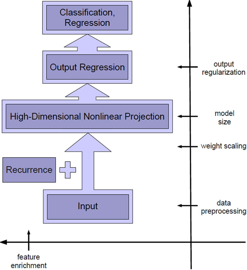
Figure 5. Machine learning view of RNs.
random projections work in these models, we compare an ELM and the corresponding reservoir network on the same tasks. We argue that the additional mixing effect of the recurrence enhances model complexity. The hypothesized effect can be visualized and evaluated on three levels: for the single feature, the learned function, and with respect to the task performance.
3.1. Recurrence Enhances Feature Complexity by Nonlinear Mixtures
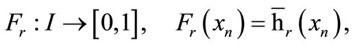
We first consider the level of a single neuron and the feature it computes in a given architecture. We define such a feature Fr as the response of the r-th reservoir neuron hr to the full range of possible inputs  from the network’s input space
 :
:
where  denotes the network’s converged attractor state (cf. Section B). The feature can easily be visualized as e.g. in Figure 6, which shows features of an ELM and a corresponding RN for the reference example of the Mexican hat data set (cf. Section C.2). For the ELM, the features are completely determined by the activation function parameters a and b of the corresponding neuron. Regardless of the specific choice of the activation function parameters, the set of possible features in an ELM (top row) is quite restricted, namely to monotonically increasing or decreasing functions: standard sigmoid functions (left), stretched or compressed shifted sigmoid functions (middle), which can approximate linear or even constant behavior (right) for an appropriate parameter choice. In contrast, recurrent connections in a corresponding reservoir network (bottom row) enhance the feature spectrum to more complex functions with possibly several local optima. Even weak recurrence with small weights gives this effect without any tuning. The effect can be seen by visual inspection but, however, is
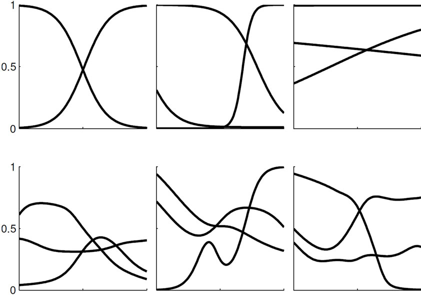
Figure 6. Exemplary features Fr generated by an ELM (top row) and a reservoir network (bottom row).
not easily be quantified and we therefore consider also the network level.
3.2. Recurrence Increases the Effective Model Complexity
3.2.1. The Mean Curvature
To assess the effective model complexity, we consider the mean curvature (MC) of the network’s output function, which directly evaluates a property of the learned model. On the one hand, this measure is closely connected to the output regularization introduced in Section A. Typical choices for regularization functionals in (9) punish high curvatures such as strong oscillations. The network’s effective model complexity is reduced [33] and the network’s output function becomes smooth through the regularized learning. On the other hand, the number of features available for learning, i.e. the network’s hidden layer size, also influences the model complexity. A small number of features decreases the model complexity and implements a kind of input regularization.
For these reasons, we measure the MC while decreasing the effective model complexity through either increasing the regularization parameter ε of the output regularization or decreasing the network size R and we expect qualitatively similar developments for varying both model selection parameters. Experiments are performed on the Mexican hat task and the default initialization parameters are shown in Section C.1. Due to the stochastic nature of parameter initialization, we average the MC over 30 networks and test each ELM and the corresponding RN for comparison.
The results shown in Figure 7 (left) reveal the expected behavior: too small network size or too strong output regularization decrease mean curvature below the necessary baseline level given by the MC of the target function, which is displayed with the dotted line. The target function can not be approximated in this case. On the other end, no regularization or very large network sizes
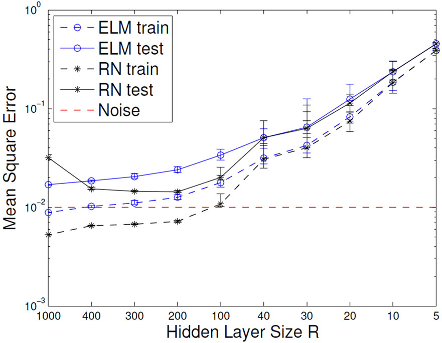
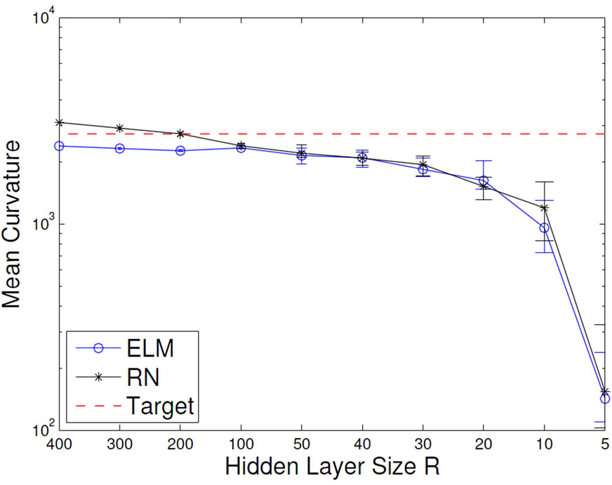
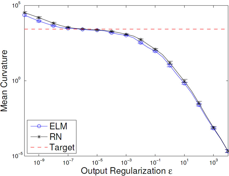
Figure 7. Development of the mean output curvature (left) and the task performance (right) of ELMs and RNs influenced by network size R (top) and output regularization strength ε (bottom).
result in a MC that is larger than the MC of the target function. This is an indication for overfitting. We also find that the ELM and the corresponding RN have very similar MC’s, except for the unregularized case, where the RN overfits more strongly. This is expected, because the more complex features of the RN provide a larger model complexity, which is favorable if the network size is limited. Note that the results for varying network size use a regularization of ε = 10–5, which is quite optimal and as such already prevents overfitting quite well. Vice versa, the results for varying ε are given for a network size of N = 100, which is clearly suitable for the task. This once more underlines that model selection and regularization are important issues.
3.2.2. The Task Performance
From the above, we expect that measuring task performance on training and test data displays a typical overfitting pattern. For small networks or too strong regularization, training and test performance are poor, for increasing regularization and for larger network size the test error reaches a minimum and then starts increasing, while the training error keeps decreasing. This is exactly the case in Figure 7 (bottom). We observe the same pattern of the RN networks for increasing network size, however, the ELM does not overfit even for large networks, if properly regularized. That is due to the limited complexity of its features and underlines the increased modeling power of the RN, which is caused by the non-linear mixing of features and also leads to a significantly better test performance. We therefore have to trade model complexity and better performance for risk of overfitting when moving from ELM to RN.
3.3. Recurrence Enhances the Spatial Encoding of Static Inputs
The results of the last section show the higher complexity of the RN in comparison to the ELM, which is caused by the non-linear mixing of features. While the exact class of features which is thereby produced is unknown, [20] introduced an approach to analyze how the inputs are represented in RNs compared to the corresponding ELMs. It is based on considering the hidden state representation  and measuring the cumulative energy content:
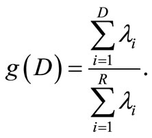
Thereby λ1 ≥ ···≥ λR ≥ 0 are the eigenvalues of the covariance matrix  corresponding to the principal components (PCs) of the network’s attractor or hidden state distribution
 . In principle, the cumulative energy content measures the increased dimensionality of the hidden data representation
  compared to the dimensionality D of the input data x. The case of g(D) < 1 implicates a shift of the input information to additional PCs, because the encoded data then spans a space with more than D latent dimensions. If g(D) < 1, no information content shift occurs, which is true for any linear transformation of data. The experiments conducted with several data sets from the UCI repository [37] showed that the cumulative energy content g(D) of the first D PCs of the attractor distribution is significantly lower for reservoir networks than for ELMs (see Figure 8). That is, a reservoir network redistributes more information in the input data onto the remaining R-D PCs than the feedforward ELM. This effect, which is only due to the recurrent connections and the respective mixing of features shows that RNs inherently hold a higher dimensional hidden data representation, which can be advantageous for the separability of input patterns and thus increases learning performance, e.g. on classification tasks.
4. Feature Regularization with Intrinsic Plasticity
In the previous section, we have shown that overfitting can occur when using an ELM and is even stronger when a corresponding RN with its richer feature set is used. Output regularization can counteract this effect, however, needs proper tuning of the regularization parameter. Hence, we propose a different route to directly tune the features of an ELM and the corresponding RN with respect to the input. A machine learning view on this idea is visualized in Figure 9. We adapt the parameters of the non-linear functions in the hidden layer by means of an unsupervised learning rule called intrinsic plasticity (IP). IP is biologically motivated and was first introduced in [29]. The idea to use IP for ELM and RN is motivated by
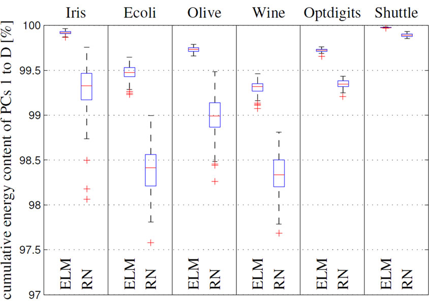
Figure 8. Results from [20]. Normalized cumulative energy content g(D) of the first D PCs tested on several classification tasks.
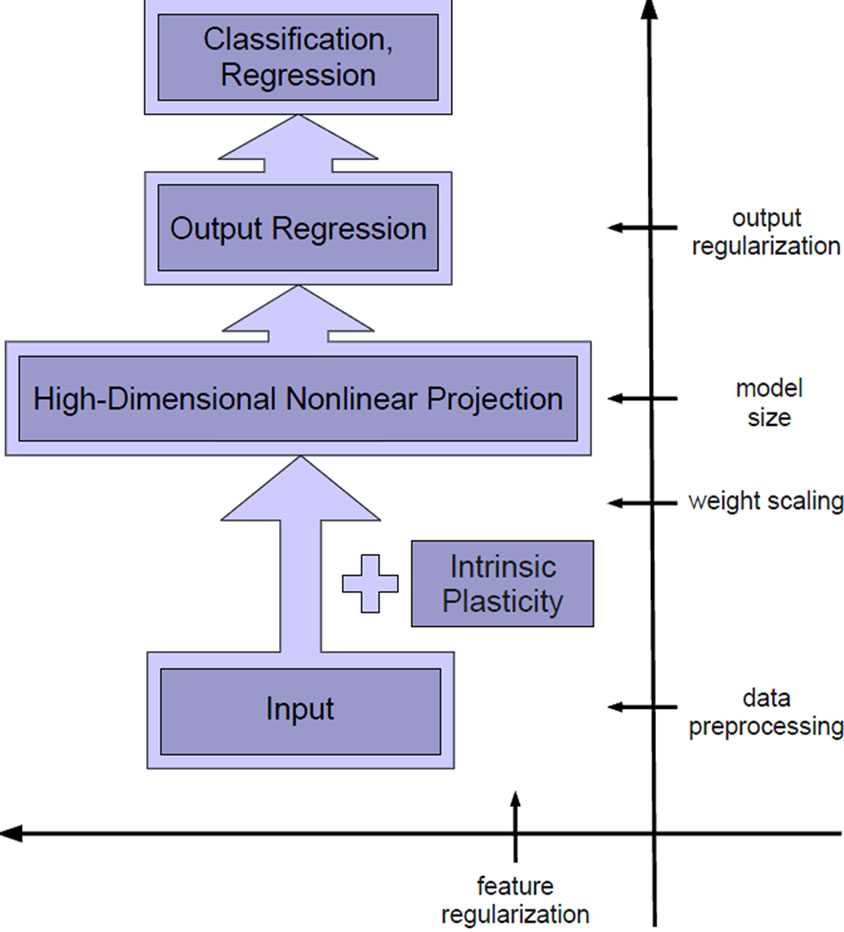
Figure 9. Machine learning view of IP-pretrained ELMs.
previous work [38,39], where IP was shown to provide robustness against both varying weight and learning parameters. We show that IP in our context works as an input regularization mechanism. Again, we analyze the resulting networks on all three levels: with respect to feature complexity, by means of the MC, and by evaluating task performance.
4.1. Intrinsic Plasticity Revisited
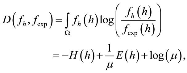
Intrinsic Plasticity (IP) was developed by Triesch in 2004 [29] as a model for homeostatic plasticity for analog neurons with Fermi-function. Its goal is to optimize the information transmission of a single neuron strictly locally by adaption of slope a and bias b of the Fermifunction such that the neurons’ outputs h become exponentially distributed. IP-learning can be derived by minimizing the Kullback-Leibler-divergence D(fh, fexp) between the output fh and an exponential distribution fexp:
 (6)
(6)
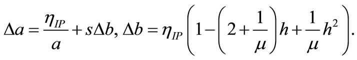
where H(h) denotes the entropy and E(h) the expectation value of the output distribution. In fact, minimization of D(Fh, Fexp) in Eq. (6) for a fixed E(h) is equivalent to entropy maximization of the output distribution. For small mean values, i.e. μ ≈ 0.2, the neuron is forced to respond strongly only for a few input stimuli. The following online update equations for slope and bias-scaled by the step-width ηIP- are obtained:
 (7)
(7)
The only quantities used to update the neuron’s non-linear transfer function are s, the synaptic sum arriving at the neuron, the firing rate h and its squared value h2. Since IP is an online learning algorithm, training is organized in epochs: For a pre-defined number of training epochs the network is fed with the entire training data and each hidden neuron is adapted to the network’s current input separately. Within the ELM paradigm, IP is used as a pre-training algorithm to optimize the hidden layer features before output regression is applied.
4.2. Regulating ELM Complexity through Intrinsic Plasticity
4.2.1. IP and Feature Complexity
Since IP adapts the parameters a and b of the hidden neurons’ activation function it directly influences the features generated by an ELM. Figure 10 visualizes the development of the network’s features’ shape during IP training for one dimensional inputs as it was done in Section 3. The left plot in Figure 10 shows a collection of features for a randomly initialized ELM. The features are distributed over the whole range of inputs. Through IPpretraining, the variety in the set of features is reduced (see Figure 10(b)), until the extreme case of only two features is reached (see Figure 10(c)).

Figure 10. Random features Fr (a), IP-regularized features after a few (250) epochs (b) and strong (1000) IP-regularized features (c) of an ELM.
4.2.2. IP and the Effective Model Complexity
On the network level, we evaluate model complexity again by means of the MC and the network performance on the Mexican hat regression task. We apply readout learning after each epoch to monitor the impact of IP on these measures over epochs. Learning and initialization parameters are collected in Section C.1. For illustration we choose the size of the ELMs’ hidden layer as R = 100 and the number of samples used for training as Ntr = 50 such that the ELM is prone to show overfitting and the effect of regularization can be observed clearly. The results are shown in Figure 11.
Figure 11(a) shows that the MC is decreasing with more IP epochs and thus shows a typical regularization behavior qualitatively similar to the dependency on the output regularization shown before in Figure 7 (bottom left). The optimal MC of the Mexican hat function is reached at about 300 IP-Epochs, more IP epochs further reduce the curvature such that no proper approximation of the target function is possible. Note that in contrast to networks with output regularization the MC does not fall dramatically down to zero.
The task performance shown in Figure 11(b) confirms that IP-pretraining has typical characteristics of a regularization mechanism. Low regularization strength (few IP epochs) results in low training error but high test error; over-fitting occurs. In contrast, too strong regularization (too many IP epochs) results in a degenerated behavior indicated by simultaneously high training and test error. The optimal regularization strength can be found in between these areas.
In Figure 11(c) we add a further analysis of the performance by decomposing the errors into integrated squared bias and integrated variance during IP training (cf. Section A). It shows that the variance of the outputs decreases with the amount of IP epochs, while the bias is first constant and then increases rapidly, when the model complexity starts to degenerate. The observed trade-off between these quantities indicates the similarities to regularization processes [25].
Finally, we plot 30 trained ELMs for non IP, medium IP epochs and too many IP epochs each in Figure 12.
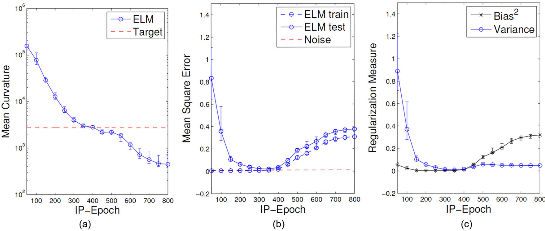
Figure 11. Mean curvature (a), training and test error (b) and bias and variance decomposition measures (c) during IP training of ELMs on the Mexican hat regression task.
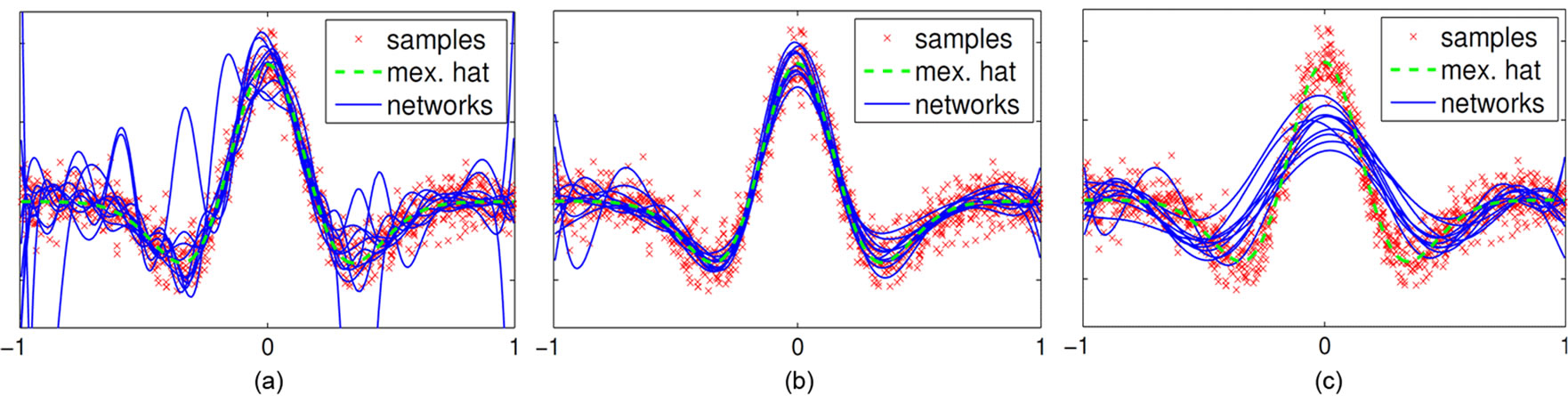
Figure 12. Outputs y of a single ELM trained with 0 (a), 250 (b), and 1000 (c) IP-epochs on different folds of the Mexican hat regression task.
The ELMs without IP-training (a) clearly show the typical oscillations due to over-fitting; a suited number of IP pre-training epochs (b) leads to constantly good results, whereas too long IP pre-training (c) tends to reduce the model complexity inappropriately so that the mapping is not accurately approximated anymore. The set of corresponding features is shown in Figure 10, respectively.
The experiments in this section clearly reveal the regulatory nature of IP as a task-specific feature regularization for ELMs.
5. Intrinsic Plasticity in Combination with Recurrence
We now show that the combination of recurrence and IP can achieve a balance between task-specific regularization by means of IP and a large modeling capability by means of recurrence. Whereas this is interesting from a theoretical point of view, it turns out that this combination also strongly enhances robustness of the performance with respect to other model selection parameters and eases the burden to perform grid-search or other optimization of those. To obtain comparable results to the experiments performed in the last sections, we add recurrent connections to the hidden layer of the ELMs to obtain the corresponding RN (see Figure 13 for illustration of the corresponding machine learning viewpoint). Recurrent weights are randomly drawn from a uniform distribution in [–1, 1] with a density of ρ = 0.1. Only at tractor states are used for IP-learning, i.e. the networks are iterated until convergence for constant input as described by Alg. 1 in Section B before applying the IP learning-step given by (7). We again analyze feature complexity, MC, and the performance in turn.
Feature Complexity
Figure 14 illustrates the development of the features of a reservoir network during IP training. The features are not only sigmoid anymore due to the addition of the recurrent weights. As observed in Section 4.2 during IP training the features become similar and input specific, but in contrast to ELMs (compare to Figure 10 in Section 4.2)recurrent features stay complex even after a huge amount of IP training.
Network Complexity
We repeat the experiments from the previous Section 4 with the corresponding reservoir networks instead of ELMs. The network settings are given in Section C.1. The MC development with respect to IP-training of the reservoir networks is illustrated in Figure 15 (a). Similar to the ELMs (cf. Figure 11), the RNs’ output function’s curvature decreases in the first epochs, but then stays close to the curvature of the target function without dropping to small values. This indicates that the regularization effect of IP and recurrence balance very well, in contrast to the ELM experiments where the output curvature falls significantly below the mean task curvature when regularizing to strongly for both output and feature-regularization.
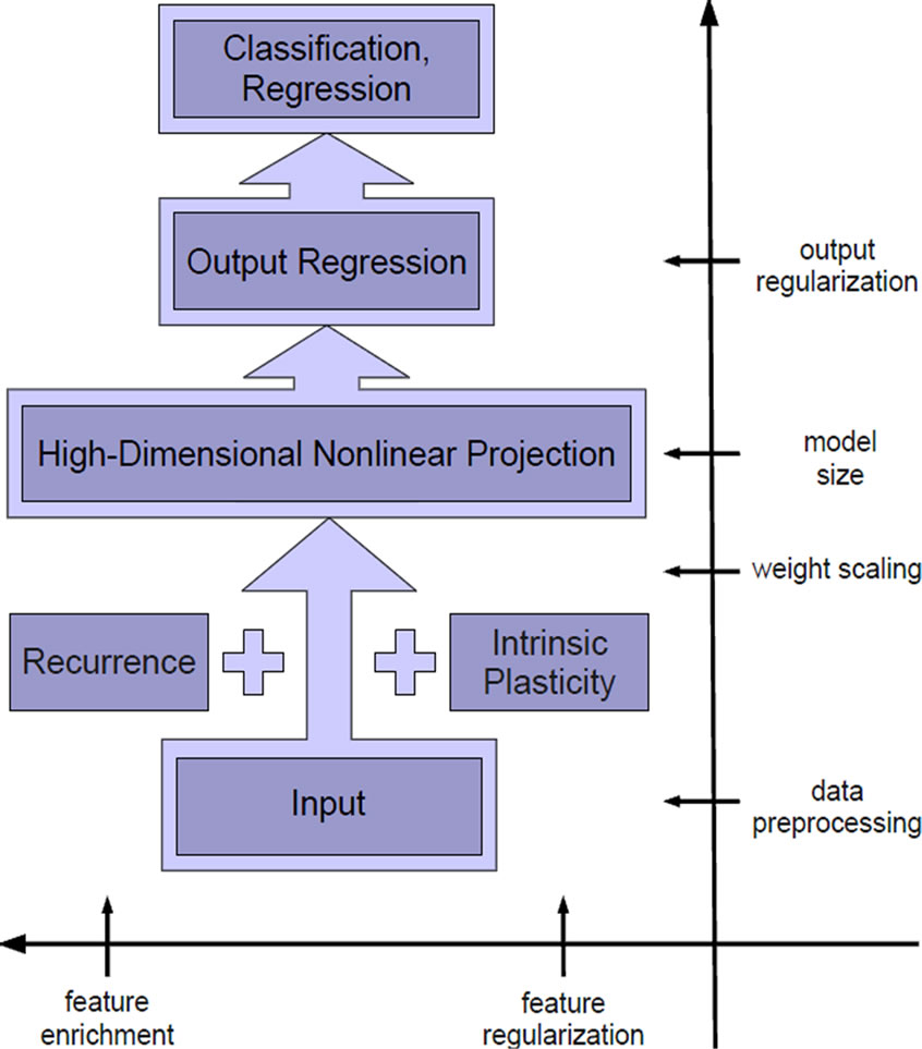
Figure 13. Machine learning view of IP-pretrained RNs.
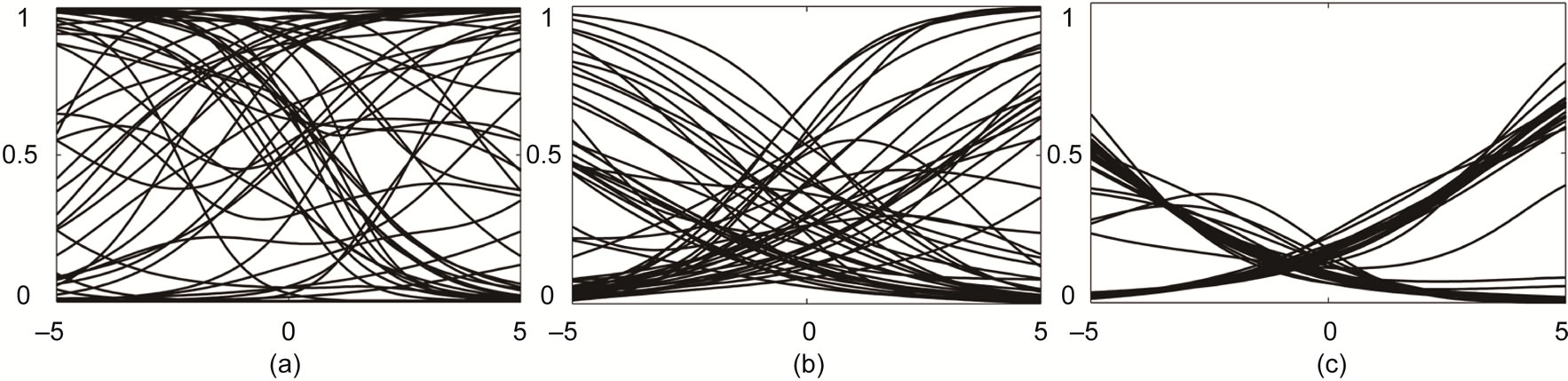
Figure 14. Random mixture of features Fr (a), IP-regularized features after a few epochs (b), and strong IP-regularized features (c) of a reservoir network.

Figure 15. Mean curvature development (a) training and test error (b) and bias-variance decomposition (c) of IP-trained reservoir networks performing the Mexican hat regression task.
Figures 15(b) and (c) show the performance and the bias/variance decomposition. The behavior of the networks show similar characteristics as the ELMs under the influence of IP (compare to Figure 11): Stronger regularization implemented by longer IP pre-training increases the generalization ability indicated by a lower test error and decreasing variance. Hence, reservoir networks still profit from the feature regularization. But in contrast to the results obtained for the ELMs, bias and test error do not increase for many IP epochs, i.e. no degeneration of the networks is observed. Obviously, the recurrent connections maintain the networks’ high mapping capabilities even in the presence of strong regularization through IP.
5.1. Increased Model Complexity for More Complex Tasks
In previous sections, we used synthetic data and a rather simple one-dimensional task to clearly state and illustrate the concepts. We now investigate the enhanced intrinsic model complexity, which is due to the addition of recurrent connections, in a more complex function approximation task where the task complexity can be controlled with a single parameter. The target function is a two-dimensional sine function (cf. Section C.3), where the frequency ω is proportional to its mean curvature and the difficulty of task.
Figure 16 shows the MSE on the training and test set for ELMs and corresponding RN, both pretrained with the same amount of IP-epochs, with respect to increasing frequency ω. The initialization parameters of the networks are stated in Section C.1. As expected, the errors increase with the frequency and at some frequency the networks can not approximate the function appropriately. This is indicated by a rapid deterioration of the performance, which occurs for the ELMs at ω ≥ 2, whereas the error for the recurrent networks does not increase strongly until ω ≥ 3. This experiment shows that the enhanced mapping capability due to the addition of recurrent connections is preserved despite the IP-training of the networks. As a result, IP-trained reservoir networks are suitable for a wider spectrum of task complexities than IP-trained ELMs.
5.2. Parameter Robustness
Picking up the discussion on model selection for the ELM in Section 2.1, we finally show that the combination of recurrence and feature regularization via IP makes the networks less dependent on the specific choice of other model selection parameters and the random initialization.
We investigate three important model selection parameters: the number of hidden neurons R, the output regularization strength ε, and the scaling of the input weights and biases. In order to show the dependency of the different approaches to the model selection parameters, a predefined parameter space will be sampled by initializing 30 networks at 100 given points. The bias scaling and input scaling is drawn from the uniform distribution in [1, 20], while the hidden layer size is uniformly drawn from [10, 11, ···, 300]. The output regularization is chosen from [10–6, 102]. The recurrent weights of the RNs where uniformly drawn from [–0.2, 0.2] with a density of ρ = 0.1. The IP-training had a fixed mean μ = 0.2 with a step-size of ηIP = 10–3.
The experiment is conducted with often used benchmark tasks from the UCI repository, see Section C.4, for which the result of the different network approaches are collected in Table 1.
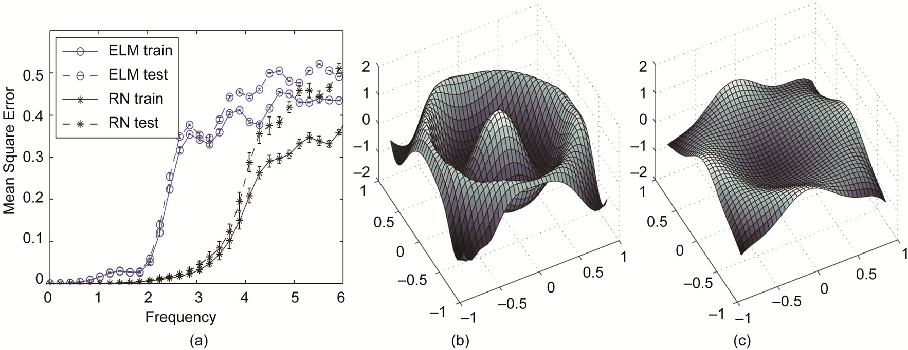
Figure 16. (a) Training and test errors for IP-pretrained ELMs and RNs for different frequencies ω of the two-dimensional sine wave approximation task; (b) and (c) Exemplary outputs of an ELM and its corresponding RN, respectively, being trained for ω = 3.
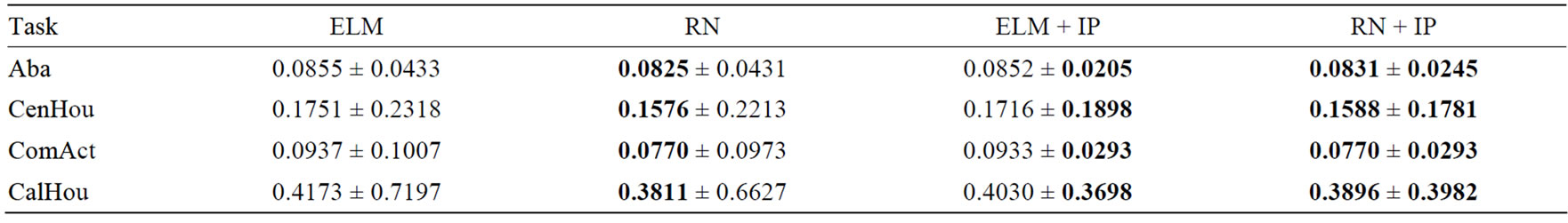
Table 1. Average test RMSEs and standard deviations for the different network settings on regression tasks from the UCI repository [37].
The table shows that IP trained RN’s perform better than purely random initialized ELMs on average and with a lower variance. The results is fully consistent with the previous chapters. On the one hand, the networks trained with IP have a significantly lower variance in the performance than the randomly initialized networks. This is due to the feature regularization. On the other hand, networks with recurrent weights perform better on average indicating that the mapping capability is enhanced. Both mechanisms, the feature regularization and the nonlinear mixture of random features are exploited and have a positive effect on the task performance.
Figure 17 additionally shows how the networks gen eralization performance is enhanced and much more robust after the addition of recurrent weights and IP training on the abalone regression task [37].
The plot shows networks, where the same parameters were varied as in the previous experiment. The networks had a R = 80 neurons hidden layer, a weight decay of ε = 10–6 and the input initialization range [–10, 10]. The parameters in Figure 17 are independently changed.
The networks show a high robustness against parameter change after the addition of recurrent weights and IP training.
6. Discussion
In this work, we give a comprehensive account on the modeling power of the extreme learning machine and show that overfitting, regularization and model selections are important issues also for this random projection approach. As depicted in Figure 18, we then demonstrate two ways to affect an ELM’s model complexity by directly modifying its features: either through feature regularization by intrinsic plasticity or by adding recurrent connections, which puts us into the domain of reservoir networks. Combining these two approaches, we achieve a large performance robustness against the chosen model selection and output regularization parameter. With an eye on practical application, this is clearly a highly desirable property for an approach that is based on random features.
The paper has also some interesting theoretical implications. We start our discussion with the intrinsic plasticity adaptation rule, which was introduced in [29] and has been used in the context of recurrent networks before [38-40]. Already in [38], a regularization effect was hypothesized, but not clearly shown. A proper analysis of IP from a machine learning point of view has since then not yet been provided in the literature. The analysis in this contribution by means of the bias/variance decomposition and the MC clearly reveals that IP works as a feature regularization mechanism. The duration of the IP-pretraining thereby controls regularization strength.
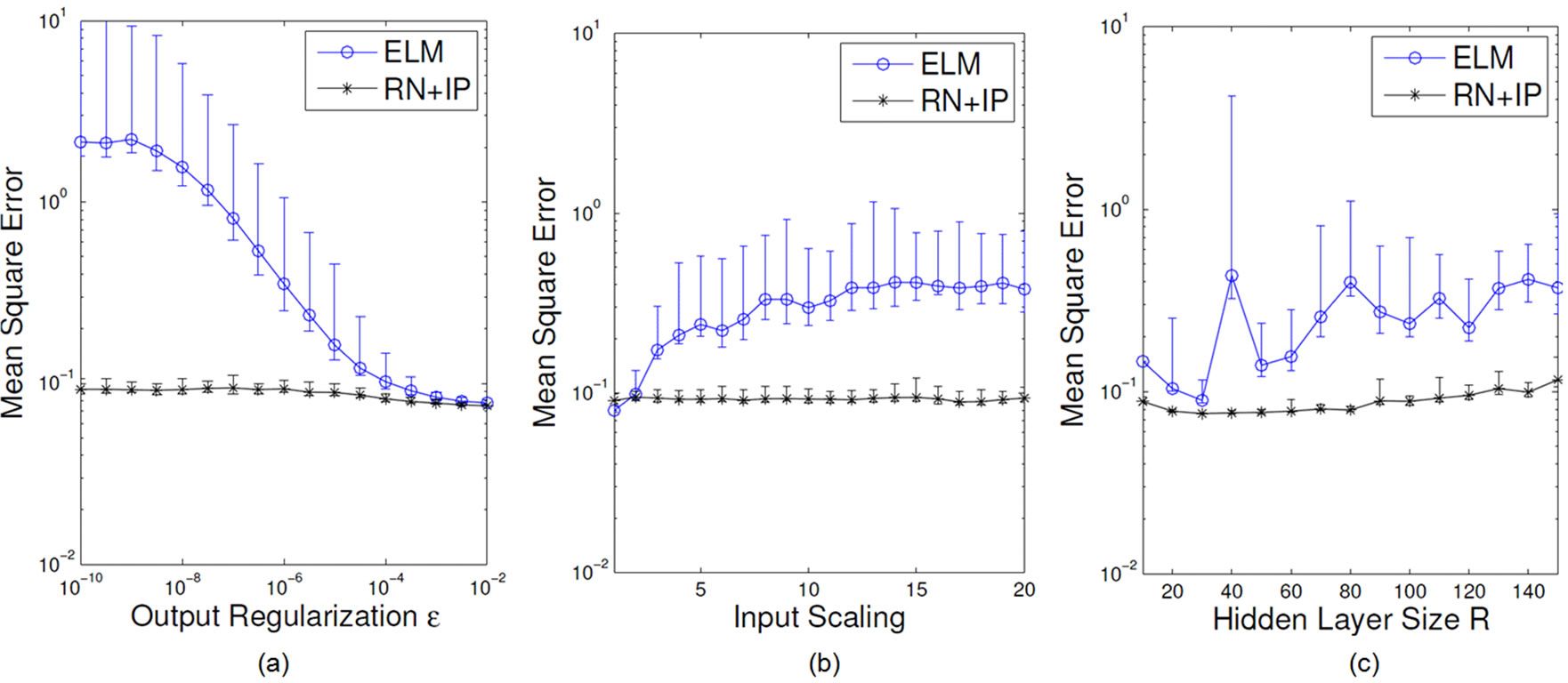
Figure 17. Test error of purely random initialized ELMs and IP-pretrained reservoir networks depending on output regularization (a), input scaling (b) and network size (c).
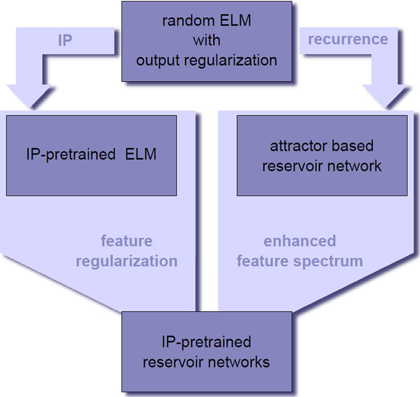
Figure 18. Sketch of argumentation.
Thus, with the usage of IP-pretraining the effective model complexity can be adjusted and overfitting can be avoided.
It is not surprising that the representational power of a RN corresponding to an ELM is larger because the recurrence enriches the feature spectrum by non-linear mixtures. It is surprising, however, that the direct combination of input-regularization by IP and recurrence results in a very good balance between these opposing mechanisms of complexity reduction and complexity enhancement without the need for further measures. As a result IP-pretrained reservoir networks are robust against the specific choice of model selection and learning parameters, like network size and output regularization parameter. Additionally, the influence of the stochastic nature of random projections in the hidden layer is reduced in the sense that the task specific performance of IP-pretrained reservoir networks is significantly less dependent on the random initialization of a network than for purely random ELMs. The variance over different network initializations is negligible and a very good performance is reached with a very high probability without much search (cf. Section 5.2). This is a rare example that the combination of several approaches is directly possible without introducing hyper parameters or additional arbitration.
A very interesting question is, what the presented results imply for the analysis of reservoir networks that are operated not in attractor mode. In [38], Steil recommended to use online IP as an optimization method for reservoirs also for the processing of temporal data. In such an continuously adapted network, which is driven by a temporal input, the features vary continuously. Even though non-constant, the non-linear mixing occurs in a similar way as demonstrated here. It is more difficult to transfer the regularization effect of IP, because in a continuously plastic network the IP adaptation tunes the features to the varying distribution. If slowly changing, IP tunes the features towards the average distribution, but the recurrent effects can not be quantified. The empirical results presented in [38] suggest that nevertheless IP is able to achieve a good approximation of the optimal output distribution. If this is the case, we predict that IP acts as a feature regularizer in a very similarly way as demonstrated here. The verification of this is beyond the scope of this work and left to a future investigation.
REFERENCES
- Y. Miche, B. Schrauwen and A. Lendasse, “Machine Learning Techniques Based on Random Projections,” In Proceedings of European Symposium on Artificial Neural Networks, Bruges, April 2010, pp. 295-302.
- Y.-H. Pao, G.-H. Park and D. J. Sobajic, “Learning and Generalization Characteristics of the Random Vector Functional-Link Net,” Neurocomputing, Vol. 6, No. 2, 1994, pp. 163-180. doi:10.1016/0925-2312(94)90053-1
- D. S. Broomhead and D. Lowe, “Multivariable Functional Interpolation and Adaptive Networks,” Complex Systems, Vol. 2, No. 1, 1988, pp. 321-355.
- G.-B. Huang, Q.-Y. Zhu and C.-K. Siew, “Extreme Learning Machine: A New Learning Scheme of Feedforward Neural Networks,” Proceedings of International Joint Conferences on Artificial Intelligence, Budapest, July 2004, pp. 489-501.
- G.-B. Huang, Q.-Y. Zhu and C.-K. Siew, “Extreme Learning Machine: Theory and Applications,” Neurocomputing, Vol. 70, No. 1-3, 2006, pp. 489-501.
- L. P. Wang and C. R. Wan, “Comments on the Extreme Learning Machine,” IEEE Transactions on Neural Networks, Vol. 19, No. 8, 2008, pp. 1494-1495.
- M. Lukosevicius and H. Jaeger, “Reservoir Computing Approaches to Recurrent Neural Network Training,” Computer Science Review, Vol. 3, No. 3, 2009, pp. 127- 149.
- M. Hermans and B. Schrauwen, “Recurrent Kernel Machines: Computing with Infinite Echo State Networks,” Neural Computation, Vol. 24, No. 6, 2011, pp. 104-133.
- D. Verstraeten, B. Schrauwen and D. Stroobandt, “Reservoir-Based Techniques for Speech Recognition,” International Joint Conference on Neural Networks, Vancouver, 16-21 July 2006, pp. 1050-1053.
- M. D. Skowronski and J. G. Harris, “Automatic Speech Recognition Using a Predictive Echo State Network Classifer,” Neural Networks, Vol. 20, No. 3, 2007, pp. 414-423. doi:10.1016/j.neunet.2007.04.006
- E. A. Antonelo, B. Schrauwen and D. Stroobandt, “Event Detection and Localization for Small Mobile Robots Using Reservoir Computing,” Neural Networks, Vol. 21, No. 6, 2008, pp. 862-871.
- M. Rolf, J. J. Steil and M. Gienger, “Effcient Exploration and Learning of Full Body Kinematics,” IEEE 8th International Conference on Development and Learning, Shanghai, 5-7 June 2009, pp. 1-7.
- R. F. Reinhart and J. J. Steil, “Reaching Movement Generation with a recurrent neural network based on Learning Inverse Kinematics for the Humanoid Robot Icub,” Proceedings of IEEE-RAS International Conference on Humanoid Robots, Paris, 7-10 December 2009, pp. 323-330. doi:10.1109/ICHR.2009.5379558
- P. Buteneers, B. Schrauwen, D. Verstraeten and D. Stroobandt, “Real-Time Epileptic Seizure Detection on IntraCranial Rat Data Using Reservoir Computing,” Advances in Neuro-Information Processing, Vol. 5506, 2009, pp. 56-63.
- B. Noris, M. Nobile, L. Piccinini, M. Berti, M. Molteni, E. Berti, F. Keller, D. Campolo and A. Billard, “Gait Analysis of Autistic Children with Echo State Networks,” Workshop on Echo State Networks and Liquid State Machines, Whistler, December 2006.
- A.F. Krause, B.Bläsing, V.r Dürr and T. Schack, “Direct Control of an Active Tactile Sensor Using Echo State Networks,” Human Centered Robot Systems, Vol. 6, 2009, pp. 11-21.
- M. J. Embrechts and L. Alexandre, “Reservoir Computing for Static Pattern Recognition,” Proceedings of European Symposium on Artificial Neural Networks, Bruges, April 2009, pp. 245-250.
- X. Dutoit, B. Schrauwen and H. Van Brussel, “NonMarkovian Processes Modeling with Echo State Networks,” Proceedings of European Symposium on Artificial Neural Networks, Bruges, April 2009, pp. 233-238.
- F. R. Reinhart and J. J. Steil, “Attractor-Based Computation with Reservoirs for Online Learning of Inverse Kinematics,” Proceedings of European Symposium on Artificial Neural Networks, Bruges, April 2009, pp. 257-262.
- C. Emmerich, R. F. Reinhart and J. J. Steil, “Recurrence Enhances the Spatial Encoding of Static Inputs in Reservoir Networks,” Proceedings of the International Conference on Artificial Neural Networks (ICANN), Thessaloniki, September 2010, Vol. 6353, pp. 148-153. doi:10.1007/978-3-642-15822-3_19
- G. Feng, G.-B. Huang, Q. P. Lin and R. Gay, “Error Minimized Extreme Learning Machine with Growth of Hidden Nodes and Incremental Learning,” IEEE Transactions on Neural Networks, Vol. 20, No. 8, 2009, pp. 1352-1357.
- G.-B. Huang, L. Chen and C.-K. Siew, “Universal Approximation Using Incremental Constructive Feedforward Networks with Random Hidden Nodes,” IEEE Transactions on Neural Networks, Vol. 17, No. 4, 2006, pp. 879- 892. doi:10.1109/TNN.2006.875977
- Y. Miche, A. Sorjamaa, P. Bas, O. Simula, C. Jutten and A. Lendasse, “OPELM: Optimally Pruned Extreme Learning Machine,” IEEE Transactions on Neural Networks, Vol. 21, No. 1, 2009, pp. 158-162. doi:10.1109/TNN.2009.2036259
- A. N. Tikhonov, “Solution of Incorrectly Formulated Problems and the Regularization Method,” W. H. Winston, Washington DC, 1977.
- S. Geman, E. Bienenstock and R. Doursat, “Neural Networks and the Bias/Variance Dilemma,” Neural Computation, Vol. 4, No. 1, 1992, pp. 1-58.
- F. Girosi, M. Jones and T. Poggio, “Regularization Theory and Neural Networks Architectures,” Neural Computation, Vol. 7, No. 2, 1995, pp. 219-269. doi:10.1162/neco.1995.7.2.219
- W. Y. Deng, Q. H. Zheng and L. Chen, “Regularized Extreme Learning Machine,” Proceedings of IEEE Symposium on Computational Intelligence and Data Mining, Nashville, 30 March-2 April 2009, pp. 389-395. doi:10.1109/CIDM.2009.4938676
- B. Schrauwen, D. Verstraeten and J. Van Campenhout, “An Overview of Reservoir Computing: Theory, Applications and Implementations,” Proceedings of European Symposium on Artificial Neural Networks, Bruges, 2005, pp. 471-482.
- J. Triesch, “A Gradient Rule for the Plasticity of a Neuron’s Intrinsic Excitability,” Proceedings of International Conference on Artificial Neural Networks, Warsaw, September 2005, pp. 65-79.
- N.-Y. Liang, G. B. Huang, P. Saratchandran and N. Sundararajan, “A Fast and Accurate Online Sequential Learning Algorithm for Feedforward Networks,” Proceedings of IEEE Transactions on Neural Networks, Vol. 17, No. 6, 2006, pp. 1411-1423.
- Q. Zhu, A. Qin, P. Suganthan and G.-B. Huang, “Evolutionary Extreme Learning Machine,” Pattern Recognition, Vol. 38, No. 10, 2005, pp. 1759-1763.
- V. N. Vapnik, “The Nature of Statistical Learning Theory,” Springer-Verlag Inc., New York, 1995.
- C. M. Bishop, “Training with Noise Is Equivalent to Tikhonov Regularization,” Neural Computation, Vol. 7, 1994, pp. 108-116.
- C. M. Bishop, “Pattern Recognition and Machine Learning,” Springer, New York, 2007.
- K. Neumann and J. J. Steil, “Optimizing Extreme Learning Machines via Ridge Regression and Batch Intrinsic Plasticity,” Neurocomputing, 2012, in Press. doi:10.1016/j.neucom.2012.01.041
- M. Rolf, J. J. Steil and M. Gienger, “Learning Exible Full Body Kinematics for Humanoid Tool Use,” International Conference on Emerging Security Technologies, Canterbury, 6-7 September 2010, pp. 171-176.
- A. Frank and A. Asuncion, “Uci Machine Learning Repository,” Amherst, 2010.
- J. J. Steil, “Online Reservoir Adaptation by Intrinsic Plasticity for Backpropagation—Decorrelation and Echo State Learning,” Neural Networks, Vol. 20, No. 3, 2007, pp. 353-364. doi:10.1016/j.neunet.2007.04.011
- B. Schrauwen, M. Wardermann, D. Verstraeten, J. J. Steil and D. Stroobandt, “Improving Reservoirs Using Intrinsic Plasticity,” Neurocomputing, Vol. 71, No. 7-9, 2008 pp. 1159- 1171.
- J. Triesch, “The combination of stdp and Intrinsic Plasticity Yields Complex Dynamics in Recurrent Spiking Networks,” Proceedings of International Conference on Artificial Neural Networks, Athens, 2006, pp. 647-652.
- A. N. Tikhonov and V. Y. Arsenin, “Solutions of Ill-Posed Problems,” Soviet Mathematics—Doklady, Vol. 4, 1963, pp. 1035-1038.
- H. Jaeger, “Adaptive Nonlinear System Identification with Echo State Networks,” Proceedings of Neural Information Processing Systems, Vancouver, September 2002, pp. 593-600.
- H. Jaeger, “The Echo State Approach to Analysing and Training Recurrent Neural Networks,” 2001.
A. Regularization Theory
When considering neural network models to minimize the quadratic error function E, prior knowledge about the learning model is injected as a regularization functional ER added to the error function:
 (8)
(8)
This approach was analyzed in [26]. An important class are the Tikhonov regularizers:
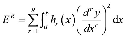 , (9)
, (9)
where hr ≥ 0 for r = 0, ···, R – 1, and hR > 0. The linear function y(x) minimizing the regularization functional is unique [41]. Here, the input interval is given by [a, b].
Since the reconstruction of a function from a finite set of data is clearly an ill-posed problem, prior knowledge of the function that has to be reconstructed is necessary in order to find a suitable solution. The most commonly used prior knowledge is that the function is smooth, such that similar inputs correspond to similar outputs [26]. Therefore, typical choices for regularization functionals in neural networks punish high curvatures, e.g. strong oscillations. We chose h2 in the functional from (9) to be
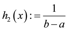
and all other equal zero. In this setting, the functional becomes the mean curvature (MC) for one-dimensional output, which we utilize to quantify regularization effects throughout this contribution.
Furthermore, the analysis of regularization mechanisms can be supported by the decomposition of the network’s error function into integrated bias and variance [25]. Whereas the former determines the network’s ability to capture the structure in the data, the latter quantifies its sensitivity to the choice of a particular training data set. The best predictive capability is given, when the optimal balance between bias and variance is reached. This sliding trade-off between both properties is characteristic for regularization methods [34] and is therefore also used in this paper to quantify regularization effects.
Weight Decay or Ridge Regression. In the context of reservoir computing and ELMs, a simple variant of the Tikhonov regularization approach [24] has become very popular to obtain networks with good generalization properties [33]. The assumption of a Gaussian prior for the learning parameters Wout leads to the new error function punishing the growth of the network’s output weights quadratically:
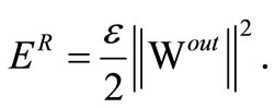
This process is called weight decay. The optimal solution in combination with linear regression is given in Equation (3) and is also known as ridge regression. It is very easy to implement and involves no additional computational costs in the batch linear regression. It is therefore a standard method employed for both ELM [27,35] and reservoir networks [7,28].
B. Attractor Based Reservoir Computing
Adding recurrent connections to the hidden layer of an ELM converts it to a corresponding reservoir network. The network state is then governed by discrete dynamics
 (10)
(10)
 (11)
(11)
with an additional randomly initialized weight matrix Wres collecting the inner reservoir connections. Inspired by biology and aiming at a reduction of computational costs often a sparsely connected reservoir is preferred. This rather simple technique has proven to work well on a variety of tasks [42]. For static mapping tasks the original approach is substituted by attractor-based computation: We map the network’s inputs xk to the related attractor states  of the reservoir rather than to the instantaneous reservoir response h(k). This is done by clamping the input neurons to the current input pattern xk until the network state change
 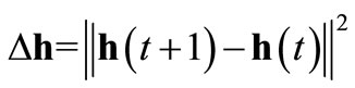 approaches zero as summarized in Alg. 8. Please note that besides this algorithm also other approaches exist to check, whether the network state is converged to an attractor state or not. For instance, in [19] the author already adopted the Hopfield energy to monitor the network convergence.
It is worth mentioning that global stability is a prerequisite for attractor based reservoir computing and it must hold that the network always converges to a fixed-point attractor. The existence of these attractors strongly depends on the algebraic properties of the reservoir weight matrix Wres. For standard echo state networks, where f = tanh, Jaeger proposed to scale the spectral radius λmax of the reservoir matrix Wres to a certain value before training the network [43]. Thereby, λmax denotes the largest amongst the absolute eigenvalues of Wres. To obtain a suitable attractor based network, the reservoir weights can be scaled such that λmax < 1, which is related to the Lipschitz constant of the hyperbolic tangens. Note, that from a mathematical point of view λmax < 1 is a necessary condition not a sufficient one. To ensure stable network dynamics, it must hold that the largest absolute singular value is less then unity. However, in practice the eigenvalue scaling is more convenient. The usage of Fermi functions slightly changes this situation because of the different Lipschitz constant of the fermi functions. In this case a convenient choice of scaling the reservoir weights is λmax < 4.
C. Experimental Setup
C.1. Parameter Settings
Table C1 contains the ranges for the uniform distributions for the random initializations and other parameters used for the experiments conducted in this paper.
C.2. Mexican Hat Regression Task
This dataset D entirely comprises N = 1000 samples. The input samples xn are drawn from a uniform distribution in [–1, 1] and the corresponding targets  are generated by the Gaussian-noised Mexican hat function
|
Algorithm 1 Convergence algorithm. |
|
Require:get external input xk Require: set t = 0, Δh=1, δ =10–6 and tmax = 1000 1: while Δh > δ and t < tmax do 2: inject external input xk into network 3: execute network iteration (10) 4: compute state change Δh = ||h(t) – h(t – 1)||2 5: t = t + 1 6: end while 7: return t |
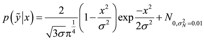
where σ = 0.2 determines the width of the Mexican hat. Though this is a low dimensional and synthetic dataset, it is often used in machine learning and serves as a proof of concept here.
In order to compile meaningful statistics in this experimental setup, for the given data set D we conduct a repeated random cross-validation for each single network: From the generated samples randomly L = 30 different cross validation folds  are created, each split up in Ntr = 50 samples for training and the remaining Nte = 950 for determining the test error. Then, we obtain the network’s performance by taking the mean of its error E over these folds.
C.3. Two-Dimensional Sine-Wave Task
The function used for the experiments has two-dimensional

Table C1. Contains the ranges for the uniform distributions for the random initializations and other parameters used for the experiments conducted in this paper.
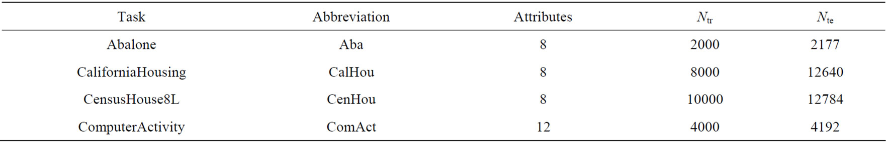
Table C2. Speciffcation of the 4 used regression data sets from the UCI machine learning repository [37].
input and one-dimensional output. Ntr = 500 samples are used for training and Nte = 100 are used for testing the networks. The results are averaged over 30 different networks with R =100 hidden neurons trained for 50 IP-epochs with ηIP = 10–3, initialized as in Table C1. The inputs are randomly drawn from the uniform distribution in [–1, 1]2. The desired outputs
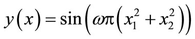
changes due to the increasing frequency ω of the mapping.
C.4. Regression Tasks
The regression tasks were taken from the UCI machine learning repository [37]. The multi-dimensional input was component-wise normalized to [–1, 1] and the onedimensional target variable to [0, 1]. Table C2 comprises information about the tasks.
NOTES
1We define an ELM to correspond to a reservoir network or vice versa, if we obtain the ELM by deleting all recurrent connections from the reservoir network.